26  标准主轴分析介绍

本部分主要来自于对 Warton 等 (2012) 和 Warton 等 (2006) 内容的理解。我姑妄言之，各位也就姑妄听之，从一个取巧的角度来讲，我觉得可以从下面的角度理解标准主轴分析：

1. 我们要比较差异，如果没有分组，我们要比较我们数据的斜率或截距是否等于一个值，例如，要研究异速生长关系，那么斜率肯定不能等于 1 吧，不然 y 和 x 是相等的生长速度，哪里来的异速生长？虽然我的文章我应该有 9 年不看了，我记忆里，是否为异速生长，就是拿斜率和 1 来比较，看其是否差异显著，当然，显著差异是我需要的。

2. 我们要分析几个分组的数据，单纯的采用线性回归是没法比较的，他们肯定是斜率和解决不同，相同那不就是同一组数据了，这样我们就要检验通过一个主轴的斜率和截距来比较，如果存在共同的斜率，那我们只能在比较截距，如果截距存在差异，某一个要高，就接着分析这个差异可能的因素就行了，这个让我毕业的文章里是用的什么，我就记不清楚了，反正就分析了什么海拔生境之类的得出的结论，我也懒得再看了，反正我用不到了。

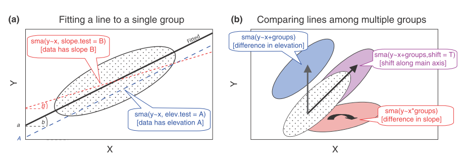
根据我多年前的记忆，SMA 的用途可以用下图进行表达：

Figure 26.1: 图示 SMATR 比较差异的方面

• 单个分组的检验，分为斜率和截距的两种：

  • 单个分组的斜率：为检验斜率是否等于某个值 b，一个简单的方法来检验就是当使用 b 作为斜率时，检验残差和轴的得分是否无关。
  • 拟合的直线经过样品的中心点 (\bar x, \bar y)，计算的截距接近正态分布，使用 t 检验来验证真正的截距是否等于某个特定值 a。

• 多个分组（多条直线）检验，是否存在共同斜率和共同截距

  • 共同斜率：共同斜率检验是检验解决是否有偏移的前提，也就是说，根据我的理解，结果存在共同斜率，我们写文章是要找差异的，找不到差异了，我们只能退而求其次，来找其截距的不同。当然，没有共同斜率，比截距也没意义。

  • 共同截距：如果存在共同斜率，我们接着要比较其是否存在共同截距。

  • 如果上面两个都相同怎么办？那还有一个检验可以来做，那就是其会沿着主轴的方向发生偏移， Warton 等 (2006) 解释了这种情况，两个物种的叶片性状在主轴方向上偏移，原因是不同营养状况下他们的叶片寿命的差异。

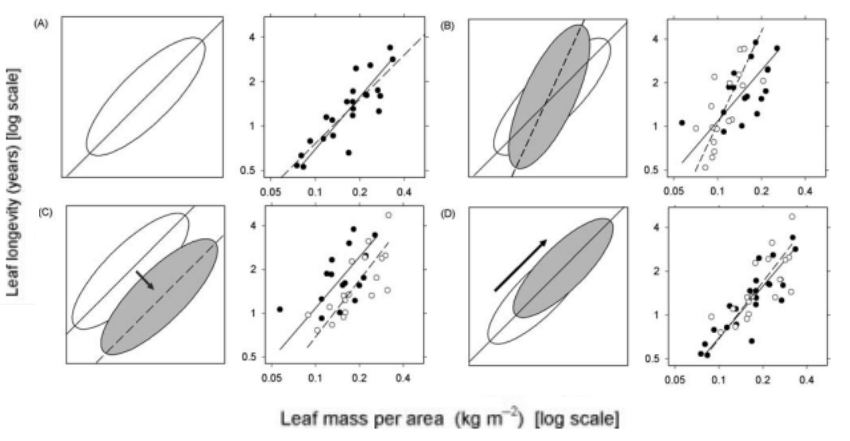
虽然 Warton 等 (2012) (Figure 26.1) 的图是彩图，但这个 Warton 等 (2006) 分开的图形更直观的解释了上面的几种情况：

• A: 检验斜率是否等于特定值
• B：检验斜率是否不同
• C：检验截距是否不同
• D：检验是否沿着主轴方向有偏移

Figure 26.2: 分开展示 SMATR 的不同检验

26.1 sma 函数的参数介绍

我还是使用软件包自带的数据，然后结合 Warton 等 (2012) 文章的内容，在尽量详细解释一下参数的意思和返回的结果，期望能使得各位不会的能够看懂。

这个软件包的最重要的函数为 sma，

sma(
  formula,
  data,
  subset,
  na.action,
  log = "",
  method = c("SMA", "MA", "OLS"),
  type = c("elevation", "shift"),
  alpha = 0.05,
  slope.test = NA,
  elev.test = NA,
  multcomp = FALSE,
  multcompmethod = c("default", "adjusted"),
  robust = FALSE,
  V = matrix(0, 2, 2),
  n_min = 3,
  quiet = FALSE,
  ...
)

其参数的意义下面就分开详细解释

26.1.1 formula

R 中的 formula 对象，通过不同的写法可以得到不同的目的，具体如下面的叙述。

单样本检验

这里但从名字上即可以看出，这应该属于上图 A 的检验，这里使用的 formula 的形式为：

• sma(y~x)，拟合 SMA 并构造真正斜率和截距的的置信区间。

• sma(y~x, slope.test = B)，检验 SMA 的斜率是否为 B。

• sma(y~x, elev.test = A)，检验 SMA 的截距是否为 A

• sma(y~x, robust = T)，使用 Huber 的 M 估计进行拟合，我对这种回归不了解，不过应该属于稳健回归的范畴，也就是帮助文档里所讲的，对野点的处理比较好。

• sma(y~x-1)， 强制从原点通过的拟合。也就是这时候没有截距的差异，或者对截距的差异不感兴趣。

多个样本检验

也就是对多个直线进行比较，有多种分组的方式：

• sma(y~x*groups)，也就是检验所有的分组有没有共同斜率。

• sma(y~x+groups, type = "elevation")，检验具有共同斜率的分组有无共同截距。

• sma(y~x*groups, type = "shift")，检验斜率是否沿着主轴方向有漂移。

• sma(y~x+groups, slope.test = "B")，检验共同斜率是否为 B。

• sma(y~x+groups, elev.test = "A")，建议共同截距是否为 A。

• sma(y~x*groups-1)，同单个样本的检验，也可以检验主轴方向的漂移。

多重比较

当 multcomp = TRUE 时，会进行各个水平间的多重比较，包括斜率、截距和沿着主轴的漂移（取决于使用的 formula）。

拟合结果

讲到这里应该继续讲函数的参数，不过我觉有必要在这里趁热打铁了，因为我觉得讲完了 formula 的几种形式，SMA 就讲完了，我们有必要把拟合结果顺带解释一下：

• coef：拟合的参数，如果有多个样品的比较，将返回模型的参数，例如检验共同斜率时各个样品或者分组的斜率

• nullcoef：零假设的参数。

• alpha：见下文的参数解释

• method：拟合使用的方法， ’MA’ 或 ’SMA’。

• intercept：拟合的线是否强制通过原点。

• call：调用 ma 或 sma 函数。

• data: 见下文的参数

• log： 见下文的参数

• variables： SMA 的线使用的变量

• origvariables：如有在拟合前有转换，转换前的变量列表

• groups：分组变量的水平

• gt：grouptest 缩写，表示分组测试的类型

• gtr：分组测试的结果

• slopetest：斜率假设检验的结果，以列表形式输出，包括 p 值、 检验统计、共同斜率 b 和置信区间 ci。

• elevtest：截距假设检验的结果，返回 p 值、t检验统计、共同截距和它的置信区间。

• slopetestdone：是否进行斜率检验

• evevtestdone：是否进行斜率的检验

• n：样品的大小

• r2：决定系数

• pval：统计结果的 p 值

• from， to：在作图 plot.sma 作图时使用的拟合线的的端点

• groupsummary：以数据框整理的分组参数

无需详细解释的参数

sma 中其他无需详细解释的参数：

• data： 包含 x 和 y 变量的数据框

• subset：用于拟合的数据框的子集，非必须选项。

• na.action: R 中对 na 值处理的方式，例如删除等。

• log：对变量使用以 10 为底的对数转换。

• method：如果等于 SMA 为标准主轴分析，MA 为主轴分析，或者选择 OLS，最小二乘法。

• type：如果多条线进行比较，我们应该选择的选项，如 elevation 或 shift。

• alpha：我们置信区间里使用的 \alpha，默认 0.05。

• slope.test: 假设检验使用的值，也就是与某一个值差异是否显著时使用。

• elev.test：与 slope.test 类似，只不过是检验截距。

• robust：如果为 TRUE，使用文件回归分析，目前仅针对单样本检验。

• V：测量误差的变异矩阵，默认无。

• n_min：一个分组最小的样品数量

• quiet：如果为 TRUE，不提示任何信息

• multcomp：如果为 TRUE，则进行多重比较

• multcompmethod： 多重比较 p 值的方法。

26.2 自带数据的例子

安装从 CRAN 上进行即可：

install.packages('smatr')

我们来使用自带的数据进行分析示例，先加载需要的软件包和数据：

library(smatr)
data(leaflife)

对于我们生态学人来说，数据浅显易懂，地点，降雨量，土壤 P 含量，叶片寿命、比叶面积几个数据：

kable(head(leaflife), caption = "示例数据{#tbl-sma-data}")

site	rain	soilp	longev	lma
1	high	high	1.1145511	125.48736
1	high	high	0.5161786	82.28108
1	high	high	0.9718517	71.02316
1	high	high	0.6722023	94.66730
1	high	high	1.0947123	119.70161
1	high	high	2.0606299	205.82589

26.2.1 单个样品的分析

我感觉单个样品的分析用的比较少，但不排除有些情况适用，我们看一下下面的结果

# 单个样品分析 --------------------------------------------------------
# 仅使用降雨和营养都是低的数据
leaf_low <- subset(leaflife, soilp == 'low' & rain == 'low')
# 仅拟合 SMA 的斜率和截距，实际很少单独用
sma(longev ~ lma, log='xy', data=leaflife)

Call: sma(formula = longev ~ lma, data = leaflife, log = "xy") 

Fit using Standardized Major Axis 

These variables were log-transformed before fitting: xy 

Confidence intervals (CI) are at 95%

------------------------------------------------------------
Coefficients:
            elevation    slope
estimate    -2.698800 1.315031
lower limit -3.224305 1.096261
upper limit -2.173295 1.577457

H0 : variables uncorrelated
R-squared : 0.4544809 
P-value : 4.0171e-10 

# 检验斜率是否与 1 差异显著
ma_test <- ma(longev ~ lma, log='xy', slope.test=1, data=leaflife)
summary(ma_test)

Call: sma(formula = ..1, data = ..4, log = "xy", method = "MA", slope.test = 1) 

Fit using Major Axis 

These variables were log-transformed before fitting: xy 

Confidence intervals (CI) are at 95%

------------------------------------------------------------
Coefficients:
            elevation    slope
estimate    -3.085214 1.492616
lower limit -3.968020 1.146777
upper limit -2.202407 2.001084

H0 : variables uncorrelated
R-squared : 0.4544809 
P-value : 4.0171e-10 

------------------------------------------------------------
H0 : slope not different from 1 
Test statistic : r= 0.3515 with 65 degrees of freedom under H0
P-value : 0.0035393 

上面的结果 H0 的 p 值仅为 0.003，也就是发生的概率太小，我们拒绝 H0，有显著差异，实际上斜率为 1.49，也很明显。

26.2.2 多个样品的分析

我们先对降雨量低的数据的性状进行分析：

low_rain <- subset(leaflife, rain == 'low') 

# SMA 单独拟合不同降雨区的数据，检验其有无共同斜率
diff_rain <- sma(longev~lma*soilp, log="xy", data = low_rain)
summary(diff_rain)

Call: sma(formula = longev ~ lma * soilp, data = low_rain, log = "xy") 

Fit using Standardized Major Axis 

These variables were log-transformed before fitting: xy 

Confidence intervals (CI) are at 95%

------------------------------------------------------------
Results of comparing lines among groups.

H0 : slopes are equal.
Likelihood ratio statistic : 3.943 with 1 degrees of freedom
P-value : 0.047076 
------------------------------------------------------------

Coefficients by group in variable "soilp"

Group: high 
            elevation     slope
estimate    -2.523634 1.1825381
lower limit -3.135266 0.9398479
upper limit -1.912003 1.4878965

H0 : variables uncorrelated.
R-squared : 0.7392636 
P-value : 1.462e-07 

Group: low 
            elevation    slope
estimate    -3.837710 1.786551
lower limit -5.291926 1.257257
upper limit -2.383495 2.538672

H0 : variables uncorrelated.
R-squared : 0.80651 
P-value : 0.00041709 

我们看到 H0 : slopes are equal 的概率是 0.047，也就是无共同斜率，图形也佐证了该点：

plot(diff_rain)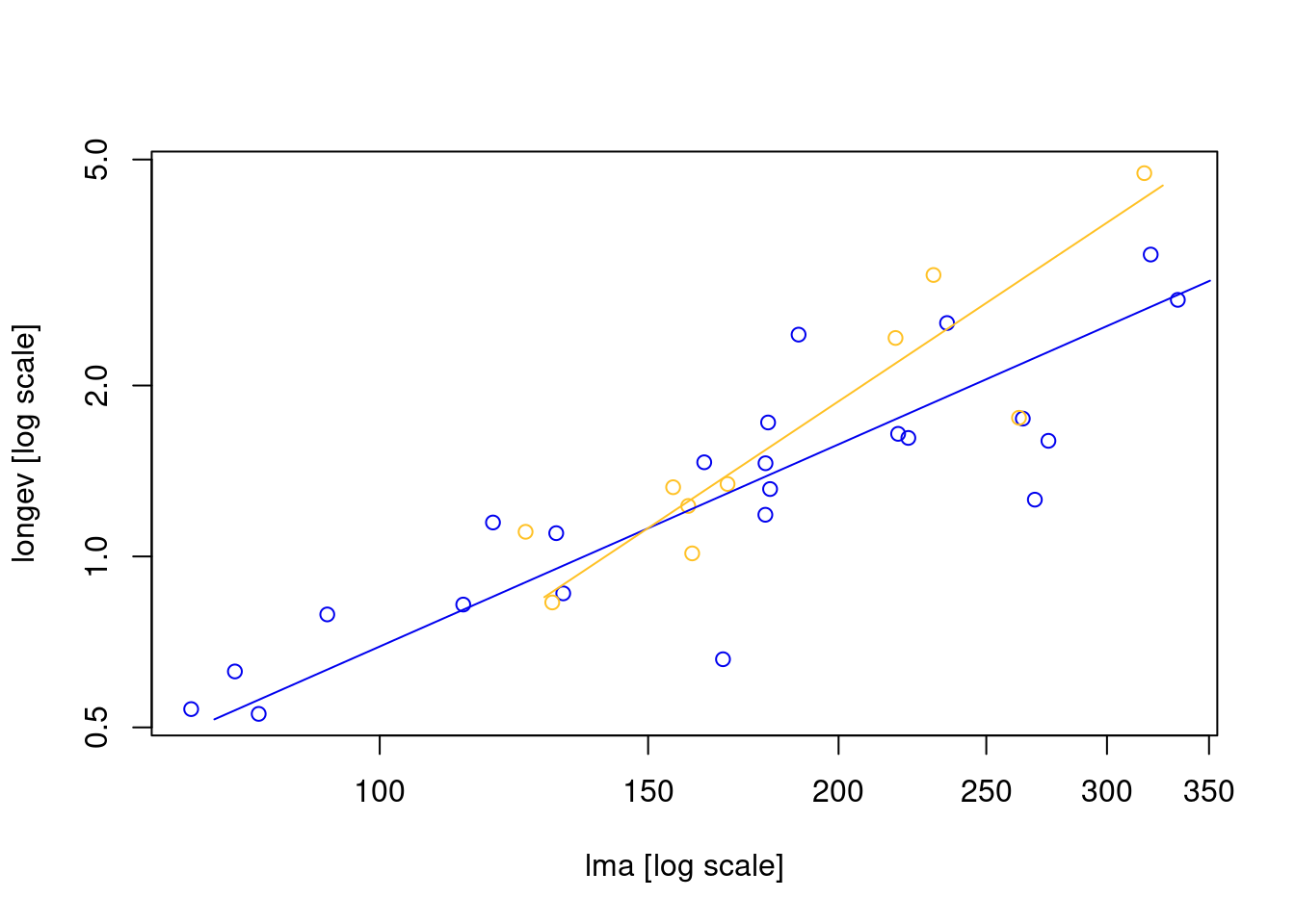

Figure 26.3: 多个分组无共同斜率

我们就无需在检验截距和延主轴的漂移了，差异足够明显。

26.2.3 多个样品无共同斜率

下面的数据时无共同斜率的情况，我就不一一解释了：

# 检查共同斜率 --------------------------------------
# 查看低土壤营养的数据
low_soilp <- subset(leaflife, soilp == 'low')

# 以降雨的高低为分组，分别拟合，检验是否有共同斜率
com_test <- sma(longev~lma*rain, log="xy", data=low_soilp )
summary(com_test)

Call: sma(formula = longev ~ lma * rain, data = low_soilp, log = "xy") 

Fit using Standardized Major Axis 

These variables were log-transformed before fitting: xy 

Confidence intervals (CI) are at 95%

------------------------------------------------------------
Results of comparing lines among groups.

H0 : slopes are equal.
Likelihood ratio statistic : 2.367 with 1 degrees of freedom
P-value : 0.12395 
------------------------------------------------------------

Coefficients by group in variable "rain"

Group: high 
            elevation     slope
estimate    -2.321737 1.1768878
lower limit -3.475559 0.7631512
upper limit -1.167915 1.8149286

H0 : variables uncorrelated.
R-squared : 0.3407371 
P-value : 0.013891 

Group: low 
            elevation    slope
estimate    -3.837710 1.786551
lower limit -5.291926 1.257257
upper limit -2.383495 2.538672

H0 : variables uncorrelated.
R-squared : 0.80651 
P-value : 0.00041709 

plot(com_test)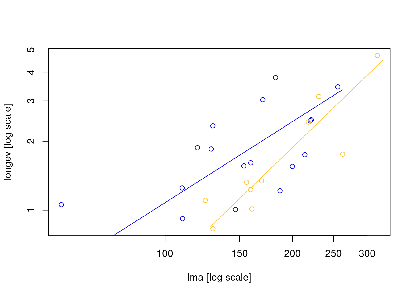

Figure 26.4: 具有共同斜率的图形

结论: H0 : slopes are equal. P 为 0.13，也就是接受 h0

# 检查斜率与 1 是否差异显著 -------------------------------------------------------------
low_soilp_b <- sma(longev~lma*rain, log="xy", slope.test=1, data=low_soilp)
summary(low_soilp_b)

Call: sma(formula = longev ~ lma * rain, data = low_soilp, log = "xy", 
    slope.test = 1) 

Fit using Standardized Major Axis 

These variables were log-transformed before fitting: xy 

Confidence intervals (CI) are at 95%

------------------------------------------------------------
Results of comparing lines among groups.

H0 : slopes are equal.
Likelihood ratio statistic : 2.367 with 1 degrees of freedom
P-value : 0.12395 
------------------------------------------------------------

H0 : common slope not different from 1 
Likelihood ratio statistic = 8.677 with 2 degrees of freedom under H0
P-value : 0.013057 

Coefficients by group in variable "rain"

Group: high 
            elevation     slope
estimate    -2.321737 1.1768878
lower limit -3.475559 0.7631512
upper limit -1.167915 1.8149286

H0 : variables uncorrelated.
R-squared : 0.3407371 
P-value : 0.013891 

H0 : slope not different from 1 
Test statistic: r= 0.1975 with 15 degrees of freedom under H0
P-value : 0.44733 

Group: low 
            elevation    slope
estimate    -3.837710 1.786551
lower limit -5.291926 1.257257
upper limit -2.383495 2.538672

H0 : variables uncorrelated.
R-squared : 0.80651 
P-value : 0.00041709 

H0 : slope not different from 1 
Test statistic: r= 0.8126 with 8 degrees of freedom under H0
P-value : 0.0042704 

# 结论： H0 : slope not different from 1 ，p 为 0.004，拒绝 h0


# 检查共同截距 -------------------------------------------------------------
low_soilp_elev <- sma(longev~lma+rain, log="xy", type = "elevation", data=low_soilp)
summary(low_soilp_elev)

Call: sma(formula = longev ~ lma + rain, data = low_soilp, log = "xy", 
    type = "elevation") 

Fit using Standardized Major Axis 

These variables were log-transformed before fitting: xy 

Confidence intervals (CI) are at 95%

------------------------------------------------------------
Results of comparing lines among groups.

H0 : slopes are equal.
Likelihood ratio statistic : 2.367 with 1 degrees of freedom
P-value : 0.12395 
------------------------------------------------------------

H0 : no difference in elevation.
Wald statistic: 6.566 with 1 degrees of freedom
P-value : 0.010393 
------------------------------------------------------------

Coefficients by group in variable "rain"

Group: high 
            elevation    slope
estimate    -3.140896 1.551400
lower limit -4.079825 1.109374
upper limit -2.201966 2.011726

H0 : variables uncorrelated.
R-squared : 0.3407371 
P-value : 0.013891 

Group: low 
            elevation    slope
estimate    -3.304865 1.551400
lower limit -4.353328 1.109374
upper limit -2.256403 2.011726

H0 : variables uncorrelated.
R-squared : 0.80651 
P-value : 0.00041709 

plot(low_soilp_elev)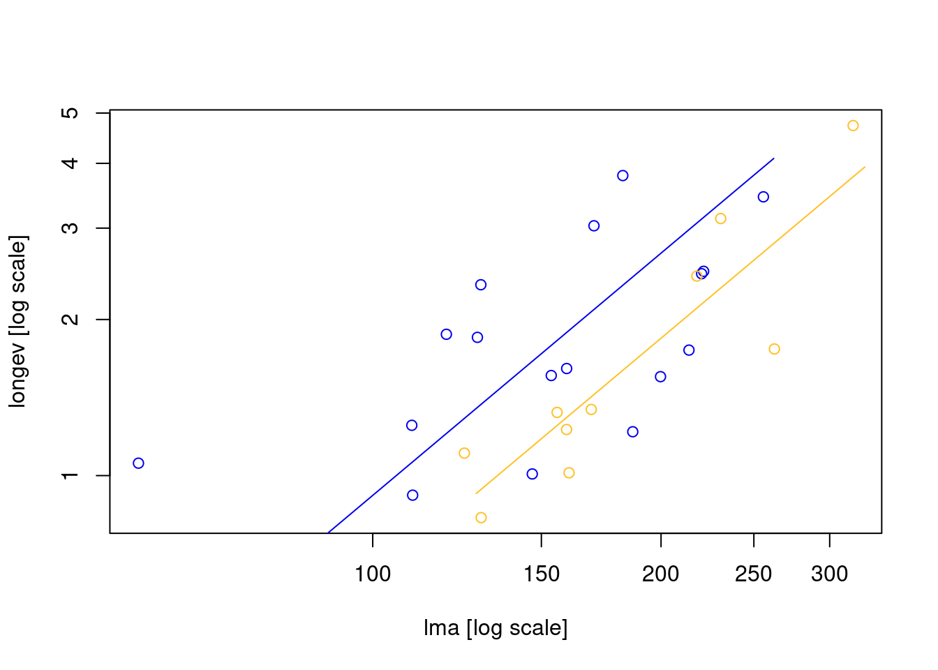

Figure 26.5: 共同截距差异显著的图形

结论： H0 : no difference in elevation. p 为 0.01 共同截距有显著差异

# 检查延主轴有无漂移 -------------------------------------------------------------
low_soilp_shift <-  sma(longev~lma+rain, log="xy", type="shift", data=low_soilp)
summary(low_soilp_shift)

Call: sma(formula = longev ~ lma + rain, data = low_soilp, log = "xy", 
    type = "shift") 

Fit using Standardized Major Axis 

These variables were log-transformed before fitting: xy 

Confidence intervals (CI) are at 95%

------------------------------------------------------------
Results of comparing lines among groups.

H0 : slopes are equal.
Likelihood ratio statistic : 2.367 with 1 degrees of freedom
P-value : 0.12395 
------------------------------------------------------------

H0 : no shift along common axis.
Wald statistic: 0.2091 with 1 degrees of freedom
P-value : 0.64745 
------------------------------------------------------------

Coefficients by group in variable "rain"

Group: high 
            elevation    slope
estimate    -3.140896 1.551400
lower limit -3.475559 1.109374
upper limit -1.167915 2.011726

H0 : variables uncorrelated.
R-squared : 0.3407371 
P-value : 0.013891 

Group: low 
            elevation    slope
estimate    -3.304865 1.551400
lower limit -5.291926 1.109374
upper limit -2.383495 2.011726

H0 : variables uncorrelated.
R-squared : 0.80651 
P-value : 0.00041709 

结论： H0 : no shift along common axis. p 为 0.64，接受 h0，无延主轴方向的漂移。

Warton, David I, Remko A Duursma, Daniel S Falster, 和 Sara Taskinen. 2012. 《smatr 3– an R package for estimation and inference about allometric lines》. Methods in Ecology and Evolution 3 (2): 257–59.

Warton, David I, Ian J Wright, Daniel S Falster, 和 Mark Westoby. 2006. 《Bivariate line‐fitting methods for allometry》. Biological Reviews 81 (2): 259–91.