第 3 章 CO₂ 响应曲线的拟合

3.1 FvCB 模型

在 plantecophys 包中使用的模型为 Farquhar, Caemmerer, and Berry (1980) 建立的 C3 植物模型 FvCB，其基于 C3 植物碳反应的三个阶段：

核酮糖-1,5-双磷酸羧化酶/加氧酶 (Rubisco)的催化下, 核酮糖-1,5-双磷酸(RuBP)与 CO₂发生羧化作用, 生成3-磷酸甘油酸(PGA)。
在腺苷三磷酸(ATP)和还原型烟酰胺腺嘌呤二核苷酸磷酸(NADPH)的作用下, PGA被还原成磷酸丙糖(TP)。每6个TP中有1个输出到细胞液中, 用于蔗糖或者淀粉的合成。
剩下的5个TP 在ATP的作用下再生为 3 个RuBP。一部分再生的 RuBP在Rubisco的催化下被氧化成PGA和2-磷酸乙醇酸, 2-磷酸乙醇酸在ATP的作用下形成PGA, 并且释放CO₂ (光呼吸)。

在光照下, C3 植物净光合速率 (A) 取决于 3 个同时存在的速率: RuBP羧化速率(Vc)、RuBP氧化速率 (或光呼吸速率, Vo)和线粒体在光照下的呼吸速率 (或明呼吸速率, Rd; 此名为了与暗呼吸速率对应和区分)。RuBP氧化过程中每结合1 mol O₂ 就会释放 0.5 mol CO₂ 。因此, 净光合速率 A 的计算为：

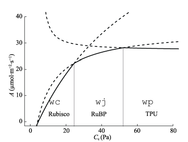
图 3.1: 光合速率的不同的限制阶段

\[\begin{equation} A\ =V_{c}\ -0.5V_{o}\ -\ R_{d} \tag{3.1} \end{equation}\]

线粒体Rd不同于暗呼吸速率(Rn )。Rn是叶片在黑暗中的线粒体呼吸速率, 随着光照的增加, 线粒体呼吸速率下降。因此 Rd < Rn 在黑暗条件下测定的叶片 CO₂ 交换速率即 Rn , 但是 Rd 的测定比较困难, 因为光照条件下 Rd 与 Vc、Vo 同时存在。Hikosaka et al. (2006) 总结了几种测定 Rd 的方法，式 (3.1) 又可表达为：

\[\begin{equation} A\ =V_{c}\ (1\ -0.5\alpha)\ R_{d} \tag{3.2} \end{equation}\]

式 (3.2) 中 \(\alpha\) 为氧化速率和羧化速率的比值，由 Rubisco 动力学常数确定：

\[\begin{equation} \begin{split} \alpha & =\frac{V_{O}}{V_{C}}\\ & = \frac{O}{C_c} \times \frac{V_{omax} K_c}{V_{cmax}K_{o}}\\ & = \frac{O}{C_{c}} \times \frac{1}{S_{\frac{c}{o}}} \end{split} \tag{3.3} \end{equation}\]

式 (3.3) 中，Cc 和 O 分别为叶绿体部位 CO₂ 和 O₂ 浓度。Cc 和 O 通常以气体摩尔分数 (\(\mu mol\text{·}mol^{-1}\) ) 或分压 (Pa) 表示, 但光合过程是在叶绿体的液相基质中发生的, 用分压表示更加恰当。Kc 与 Ko 为 Rubisco 羧化(氧化)的米氏常数, 代表了羧化(氧化)速率达到最大羧化(氧化)速率一半时的 CO₂ 和 \(O_{2}\) 浓度。是 Rubisco 特异性因子, \(S_{\frac{c}{o}}\)表示 Rubisco 对CO₂ 和 \(O_{2}\) 的偏好程度。

当 A = Rd , 即 RuBP 羧化的 CO₂ 吸收速率刚好等于 RuBP 氧化的 CO₂ 释放速率 (Vc = 2Vo，羧化时 CO₂ 提供的为 CO ) 时, \(\alpha\) = 0.5。此时叶绿体的 CO₂ 浓度就是叶绿体 CO₂ 光合补偿点, 标记为 \(\Gamma^{*}\)。即：

\[\begin{equation} \Gamma^{*}\ =\ \frac{0.5O}{S_{\frac{c}{o}}} \tag{3.4} \end{equation}\]

由公式 (3.3)和公式 (3.4)可得：

\[\begin{equation} \alpha =\frac{2\Gamma^{*}}{C_{c}} \tag{3.5} \end{equation}\]

代入公式 (3.2) 得到：

\[\begin{equation} A\ =V_{c}\ (1\ -\frac{\Gamma^{*}}{C_{c}})\ R_{d} \tag{3.6} \end{equation}\]

在 Cc 浓度很低的时候，RuBP 供应充足 (图 3.1 Rubisco 阶段)，Vc 等于 Rubisco 所能支持的羧化速率 w_c，：

\[\begin{equation} w_{c}\ =\ \frac{V_{cmax\ }C_{c}}{C_{c\ }+\ K_{c\ }(1\ +\ \frac{O}{K_{o}})} \tag{3.7} \end{equation}\]

随着 Cc 浓度的增加，Rubisco 支持的羧化速率超过了 RuBP 供应速率, Vc 受 RuBP 再生速率的限制（图 3.1 RuBP 阶段），此时 Vc 由 RuBP 的再生速率限制，而 RuBP 又由电子传递速率（J）决定，故：

\[\begin{equation} w_{j}\ =\ \frac{J\ C_{c}}{4C_{c\ }+\ 8\Gamma^{*}} \tag{3.8} \end{equation}\]

当 Cc 浓度很高，光合磷酸化超过了淀粉和蔗糖的合成速率的时候，Vc 受到 TP 利用速率（Vp）的限制（图 3.1 TPU 阶段），一般情况下，

\[\begin{equation} w_{p\ }=\ \frac{3V_{p}C_{c}}{C_{c}-\Gamma^{*}} \tag{3.9} \end{equation}\]

最终，C3 植物叶片的光合速率 A 由 w_c、w_j、w_p 的最小者决定（图 3.1 实现部分），当c > \(\Gamma^{*}\)时：

\[\begin{equation} A=min\{w_{c},w_{j,}w_{p}\}(1-\frac{\Gamma^{*}}{C_{c}})-R_{d} \tag{3.10} \end{equation}\]

3.2 CO₂ 响应曲线测量的注意事项

尽管上文对其分段性做了数学上的解释，相比来讲，不是那么通俗易懂，根据 Haworth, Marino, and Centritto (2018) 文章中的内容，我们后面两小节的内容对其进行概述：

3.2.1 分段性

与光响应曲线不同， A/Ci 曲线是分段的，这也增加了其复杂性，在其最初阶段，\(CO_2\) 浓度较低，在此阶段， Rubisco 更多的与 \(O_2\) 结合，因此，即使是较小浓度的 \(CO_2\) 的增加，也会显著提高羧化速率，我们将此阶段称之为 \(CO_2\) (Wullschleger (1993)) 限制或 Rubisco 限制 (Long and Bernacchi (2003))。净光合速率 A 与 Ci 在此阶段斜率比较陡峭，实践中往往利用计算该斜率来计算 \(V_{cmax}\)。

在较高的 \(CO_2\) 浓度下，曲线斜率开始便的平缓，作为底物的 \(CO_2\) 已经不在是限制因素，随着羧化速率达到最大，RUBP 的量成为了其限制因素，而 RUBP 的再生速率受最大电子传递速率 \(J_{max}\) 的限制。此时曲线的弯曲点由 \(V_{cmax}\) 限制转变为 \(J_{max}\)，许多研究中将饱和光下和 \(CO_2\) 浓度下测量的光合速率称之为做大光合速率(Heath et al. (2005))。而另一些研究中将最大光合速率定义为外界 \(CO_2\) 时，在饱和光强下达到的最大光合速率(Marshall and Biscoe (1980))。这些术语上的差别需要注意。

在之后，有可能继续观测到磷酸盐限制 RUBP 再生的情况，导致光合速率的下降。因为此时大量的磷酸丙糖与正磷酸盐结合，导致 ATP 合成受限制(Ellsworth et al. (2015))。这就是 TPU 限制阶段。

3.2.2 测量注意事项

尽管您的操作是严格按照说明书操作的，但说明书是指仪器的正确操作方式，无法对所有测量都采用相同设置，要获得好的测量结果，有更多的因素需要注意：

使用 LI-6400 或 LI-6800 测量 A/Ci 曲线的过程也就是控制叶室或参比室气体浓度变化的过程，只要诱导的时间足够，气孔会在相应设置的环境条件下开到足够大，这样 Ci 会随 Ca 而变化，一般来讲二者的比例为 0.7，但也可能在 0.5~0.7 间变化。

一般来讲，测量参数是在温度为 25 \(^{\circ}\)C 时获得，但实际测量过程中，因为外界温度过高或过低等无法控制叶室温度到 25 \(^{\circ}\)C，这其实并非严重的问题，因为这可以通过数学上的方法将计算参数标准化为 25 \(^{\circ}\)C 时的结果。所以，在测量时只需控制叶室温度稳定即可（通常为 20 \(^{\circ}\)C ~ 30 \(^{\circ}\)C 之间）。此外就是控制恒定的 VPD 及一个饱和光强。另外就是需要注意，开始测量之前，必须在外界环境的 \(CO_2\) 浓度下诱导足够长的时间，使光合速率达到稳定，一般需要20 ~ 30 min。对于没有稳定的光保护机制的植物，一般不建议在 50 ppm 或更低的浓度下进行设置，此时饱和光强和建议的温度下，植物没有足够的底物进行光合作用，这样会因为光化学反应的降低发生氧化性损伤。Centritto, Loreto, and Chartzoulakis (2003) 研究表明，长时间的在 50 ppm 下诱导气孔打开到最大时，可以观测到最大的气孔导度（非标准方式测量）。

对于存在干旱胁迫的测量，由于干旱会导致气孔关闭（Lauteri et al. (2014)）, 此时没有足够多的 \(CO_2\) 进入气孔，此时的测量是没有意义的，可在 50 ppm 诱导 1 h 等待气孔完全打开再快速升高 Ca 的值来进行测量（Centritto, Loreto, and Chartzoulakis (2003)）。该方法对于 \(V_{cmax}\) 不受影响而 \(J_{max}\) 降低的情况适用（Aganchich et al. (2009)）。但在某些情况下，气孔关闭速度太快，无法完成整个 A/Ci 曲线过程 (Haworth2017)（需要考虑 LI-6800 RACiR）。更重要的是，如果想采用拟合方式求 gm，那么气孔必须完全打开使叶片对 \(CO_2\) 吸收的限制降到最低。对于灌溉情况良好的植物或者土壤水分情况比较好的植物，气孔不对高于外界浓度的 Ca 的升高而响应(Haworth et al. (2015))，这可能需要更多的测量点或延长测量点的时间间隔来提高曲线的分辨率。另外，测量点的数量也要根据研究而改变，例如重点测量 Vcamx 时，50 ~ 300 ppm 的数据点要多一些，而如果研究对象是土壤磷酸盐对植物生理的限制，那么 1600 ~ 2000 ppm 的数据点要适当增多。

一个更精确的了解植物生理指标的方法是将 A/Ci 曲线改为 A/Cc 曲线，但这需要了解 gm 数据。因为 Cc 通过如下方式计算：

\[\begin{equation} C_c = C_i - \frac{A}{gm} \tag{3.11} \end{equation}\]

对于 gm 的计算，比较易操作的有几种：采用光合荧光联合测量的方式计算求得。当然也可以采用曲线拟合的方式，或者 Yin et al. (2009) 使用的方式，在低氧气体下，采用不同的光照水平求得。

此外，测量气体交换非常重要的误差来源就是气体的扩散，因为测量时，多数时间内外界气体浓度要高于叶室内的气体浓度，那么即使使用密封性非常好的材料，由外界高 \(CO_2\) 浓度气体向叶室低 \(CO_2\) 浓度气体的扩散无法避免，尤其是在连续长时间测量时该效应尤为明显，因此需要经常更换叶室垫圈。具体可以通过一些方法来校正（Flexas J and A (2007)，rodeghiero2007major），但如果采用 LI-6800 测量这将不是问题，它采用的叶室增加技术并根据测量的漏气情况对结果自动修正。

3.3 `plantecophys` 软件包

Remko A. Duursma 在2015年发表了一篇文章 Remko A. Duursma (2015)，plantecophys 是其开发的一个R包工具集，用于对叶片气体交换数据进行分析和建模。实现了如下功能：

CO₂ 响应曲线 (A-Ci curves) 的拟合、作图及模拟。
不同气孔导度模型。
根据 Cowan-Farquhar 的假设估算最适的气孔导度。
耦合气体交换模型的实现。
基于 Ci 模拟 C4 光合。
RHtoVPD：常用单位的转换（相对湿度、水汽压亏缺、露点温度）。

各参数的基本用法请参考后文内容，或官方帮助文档:

plantecophys。

3.4 LI-6400XT CO₂ 响应曲线的拟合

LI-6400XT CO₂ 响应曲线的拟合需要借助 plantecophys 的 fitaci 实现，fitaci 函数为根据 FvCB 模型对 A-Ci 曲线的测量数据进行拟合，并估算 J\(_{max}\)、V\(_{cmax}\)、R\(_{d}\)及他们的标准差，并根据 B. E. Medlyn et al. (2002) 的方法考虑了温度的影响。

3.4.1 fitaci 函数介绍

fitaci 的用法如下³：

fitaci(data, varnames = list(ALEAF = "Photo", 
  Tleaf = "Tleaf", Ci = "Ci", PPFD = "PARi", 
  Rd = "Rd"), Tcorrect = TRUE, Patm = 100, 
  citransition = NULL, quiet = FALSE, 
  startValgrid = TRUE, fitmethod = 
  c("default", "bilinear", "onepoint"), 
  algorithm = "default", fitTPU = FALSE, 
  useRd = FALSE, PPFD = NULL, Tleaf = NULL, 
  alpha = 0.24, theta = 0.85, gmeso = NULL, 
  EaV = 82620.87, EdVC = 0, delsC = 645.1013,
  EaJ = 39676.89, EdVJ = 2e+05, 
  delsJ = 641.3615, GammaStar = NULL, 
  Km = NULL, id = NULL, ...)

## S3 method for class 'acifit'
plot(x, what = c("data", "model", "none"),
     xlim = NULL, ylim = NULL, whichA = c(
       "Ac", "Aj", "Amin", "Ap"), add = FALSE,
pch = 19, addzeroline = TRUE, addlegend = 
  !add, legendbty = "o",transitionpoint = TRUE, 
linecols = c("black", "blue", "red"), lwd = c(1,
2), ...)

主要参数注释：

data：需要分析的数据，必须为 data.frame⁴。格式。
varnames：数据的表头，此处函数默认的表头为 LI-6400 的表头，分析 LI-6400 的数据时可以不用填写，直接使用默认的参数即可⁵。
Tcorrect：如果为 TRUE，那么 J\(_{max}\)、V\(_{cmax}\) 的结果为温度校正结果，若 Tcorrect = FALSE，则为测量温度下的结果。
Patm：为外界大气压。
citransition：参见详，若提供该选项，则 J\(_{max}\)、V\(_{cmax}\) 的区域则分别拟合⁶。
fitmethod：参见详解。
fitTPU：是否拟合 TPU 限制，默认为 FALSE，参见详解。
x：对于plot.acifit，x 为fitaci返回的对象，简单理解为将 fitaci 函数拟合结果赋值给一个变量，此处plot函数实际上为plot.acifit。
what：利用基础做图工具，默认为对数据和模型进行作图。
whichA：默认为对所有的光合速率进行作图（Aj=Jmax-limited (蓝色), Ac=Vcmax- limited (红色), Hyperbolic minimum (黑色)), TPU-limited rate (Ap, 如果模型有计算结果）。

其他参数请参考 FvCB 模型 Farquhar, Caemmerer, and Berry (1980) 或查看 plantecophys 的帮助文档。

3.4.1.1 fitaci函数详解

默认为非线性拟合，详见 Remko A. Duursma (2015)。
bilinear 方法使用两次线性拟合方法首先拟合 V\(_{cmax}\) 和 R\(_{d}\)，然后在拟合J\(_{max}\)，过渡点的选择为对所有数据拟合最适的点，类似 Gu et al. (2010) 的方法。该方法的优势时无论如何，都会返回拟合结果，尤其是非线性拟合失败时使用该方法，但若默认方法失败时，需首先检查是否数据存在问题。两种拟合方法的结果有轻微的差别⁷。
onepoint 参考 De Kauwe et al. (2016)。
citransition 使用时，数据将被区分为 V\(_{cmax}\) 限制（Ci < citransition ）区域，以及 J\(_{max}\) 限制 (Ci > citransition) 区域。
fitTPU：如果要计算TPU，要设置 fitTPU = TRUE，并且 fittingmethod = “bilinear”。但需要注意，当 TPU 被计算时，没有 J\(_{max}\) 限制的点的存在是可能的。TPU限制的发生是在A值不随 CO\(_{2}\) 的增加而增加时发生的，因此计算 TPU 是否有返回值，取决于测量数据是否有此情况出现。

3.5 使用 `plantecophys` 拟合 LI-6400XT CO₂ 响应曲线数据

3.5.1 数据的前处理

虽然 R 软件支持直接导入 xlsx 的数据，但因为 LI-6400XT 的数据记录文件内有其他空行或 remark 等内容，增加了处理代码的量，故而推荐将其数据先整理为如表 3.1 样式，并另存为 csv 格式⁸：

表 3.1: 推荐 LI-6400 整理后数据样式
Obs	HHMMSS	FTime	Photo	Cond	Ci	Trmmol
1	15:46:59	271.5	14.2848912	0.2730691	286.39751	2.226126
2	15:48:26	358.0	10.6562220	0.2826303	217.32002	2.292845
3	15:49:54	446.0	6.4525814	0.2909460	150.67623	2.361704
4	15:51:26	538.5	1.7971569	0.3057164	85.82530	2.459459
5	15:52:54	626.5	-0.6575974	0.3150002	53.47985	2.515992
6	15:54:50	742.5	15.4296572	0.3255415	292.56161	2.579840

3.5.2 使用示例

plantecophys 并非 base 的安装包，首次使用需要从 CRAN 安装，可以使用图形界面安装，也可以直接用命令行安装⁹，推荐同时安装依赖。

install.packages("plantecophys", dependencies = TRUE)

# 载入 plantecophys 
library("plantecophys")

# 利用read.csv读取数据文件，
# 我的路径为当前工作路径的data文件夹内
aci <- read.csv("./data/aci.csv")

# 防止可能出现的NA值
aci <- subset(aci, Obs > 0)

# 不修改默认参数对数据进行拟合
acifit <- fitaci(aci)
# 查看拟合结果的参数名称，方便导出数据使用
attributes(acifit)

## $names
##  [1] "df"             "pars"           "nlsfit"         "Tcorrect"      
##  [5] "Photosyn"       "Ci"             "Ci_transition"  "Ci_transition2"
##  [9] "Rd_measured"    "GammaStar"      "Km"             "kminput"       
## [13] "gstarinput"     "fitmethod"      "citransition"   "gmeso"         
## [17] "fitTPU"         "alphag"         "RMSE"           "runorder"      
## 
## $class
## [1] "acifit"

# 查看拟合结果
summary(acifit)

## Result of fitaci.
## 
## Data and predictions:
##            Ci      Ameas     Amodel         Ac        Aj   Ap       Rd VPD
## 5    53.47985 -0.6575974 -0.5146882 -0.3552036  0.000000 1000 0.159449 1.5
## 4    85.82530  1.7971569  1.9292621  2.0888575  5.068534 1000 0.159449 1.5
## 3   150.67623  6.4525814  6.4176037  6.5777528 12.755502 1000 0.159449 1.5
## 2   217.32002 10.6562220 10.5354626 10.6965875 17.519644 1000 0.159449 1.5
## 1   286.39751 14.2848912 14.3365887 14.4993980 20.749310 1000 0.159449 1.5
## 6   292.56161 15.4296572 14.9749157 15.1383702 20.852616 1000 0.159449 1.5
## 7   292.96456 15.7134791 15.0564801 15.2200522 20.831098 1000 0.159449 1.5
## 8   450.64285 22.2659015 23.0115187 23.1975997 25.186939 3000 0.159449 1.5
## 9   622.03873 26.5135040 27.6485003 30.4281393 27.837462 3000 0.159449 1.5
## 10  992.08737 30.3898585 30.6300461 42.3998173 30.797660 3000 0.159449 1.5
## 11 1558.96968 33.6267056 32.6638021 54.9948264 32.828110 3000 0.159449 1.5
## 12 1756.16396 33.3152783 33.0981490 58.5844507 33.261965 3000 0.159449 1.5
##       Tleaf         Cc     PPFD Patm Ci_original
## 5  31.12332   53.47934 1800.490  100    53.47985
## 4  30.99093   85.82723 1800.558  100    85.82530
## 3  30.82872  150.68265 1800.140  100   150.67623
## 2  30.63983  217.33057 1800.524  100   217.32002
## 1  30.46890  286.41186 1800.701  100   286.39751
## 6  31.26338  292.57660 1799.923  100   292.56161
## 7  31.41866  292.97963 1799.975  100   292.96456
## 8  31.54122  450.66588 1799.826  100   450.64285
## 9  31.63493  622.06640 1799.578  100   622.03873
## 10 31.73910  992.11803 1800.055  100   992.08737
## 11 31.86938 1559.00238 1800.022  100  1558.96968
## 12 31.96654 1756.19709 1799.585  100  1756.16396
## 
## Root mean squared error:  1.889701 
## 
## Estimated parameters:
##         Estimate Std. Error
## Vcmax  49.261616  1.5152405
## Jmax  126.620537  2.2816267
## Rd      0.159449  0.4001302
## Note: Vcmax, Jmax are at 25C, Rd is at measurement T.
## 
## Curve was fit using method:  default 
## 
## Parameter settings:
## Patm = 100
##  alpha = 0.24
##  theta = 0.85
##  EaV = 82620.87
##  EdVC = 0
##  delsC = 645.1013
##  EaJ = 39676.89
##  EdVJ = 2e+05
##  delsJ = 641.3615
## 
## Estimated from Tleaf (shown at mean Tleaf):
## GammaStar =  58.61138 
## Km =  1223.279

acifit_linear <- fitaci(aci,  fitmethod = "bilinear", quiet = TRUE)
summary(acifit_linear)

## Result of fitaci.
## 
## Data and predictions:
##            Ci      Ameas     Amodel         Ac        Aj   Ap        Rd VPD
## 5    53.47985 -0.6575974 -0.7389447 -0.3560483  0.000000 1000 0.3828608 1.5
## 4    85.82530  1.7971569  1.7108198  2.0938246  5.138366 1000 0.3828608 1.5
## 3   150.67623  6.4525814  6.2098476  6.5933940 12.931333 1000 0.3828608 1.5
## 2   217.32002 10.6562220 10.3375299 10.7220229 17.761317 1000 0.3828608 1.5
## 1   286.39751 14.2848912 14.1477696 14.5338762 21.035722 1000 0.3828608 1.5
## 6   292.56161 15.4296572 14.7876514 15.1743678 21.139657 1000 0.3828608 1.5
## 7   292.96456 15.7134791 14.8694171 15.2562440 21.117718 1000 0.3828608 1.5
## 8   450.64285 22.2659015 22.8464806 23.2527613 25.533374 3000 0.3828608 1.5
## 9   622.03873 26.5135040 27.8030690 30.5004944 28.220254 3000 0.3828608 1.5
## 10  992.08737 30.3898585 30.8295808 42.5006398 31.221072 3000 0.3828608 1.5
## 11 1558.96968 33.6267056 32.8913778 55.1255986 33.279305 3000 0.3828608 1.5
## 12 1756.16396 33.3152783 33.3316070 58.7237587 33.719013 3000 0.3828608 1.5
##       Tleaf         Cc     PPFD Patm Ci_original
## 5  31.12332   53.47911 1800.490  100    53.47985
## 4  30.99093   85.82701 1800.558  100    85.82530
## 3  30.82872  150.68244 1800.140  100   150.67623
## 2  30.63983  217.33037 1800.524  100   217.32002
## 1  30.46890  286.41167 1800.701  100   286.39751
## 6  31.26338  292.57641 1799.923  100   292.56161
## 7  31.41866  292.97944 1799.975  100   292.96456
## 8  31.54122  450.66572 1799.826  100   450.64285
## 9  31.63493  622.06656 1799.578  100   622.03873
## 10 31.73910  992.11823 1800.055  100   992.08737
## 11 31.86938 1559.00260 1800.022  100  1558.96968
## 12 31.96654 1756.19733 1799.585  100  1756.16396
## 
## Root mean squared error:  2.013045 
## 
## Estimated parameters:
##          Estimate Std. Error
## Vcmax  49.3787547  3.4815555
## Jmax  128.5546403         NA
## Rd      0.3828608  0.4697008
## Note: Vcmax, Jmax are at 25C, Rd is at measurement T.
## 
## Curve was fit using method:  bilinear 
## 
## Parameter settings:
## Patm = 100
##  alpha = 0.24
##  theta = 0.85
##  EaV = 82620.87
##  EdVC = 0
##  delsC = 645.1013
##  EaJ = 39676.89
##  EdVJ = 2e+05
##  delsJ = 641.3615
## 
## Estimated from Tleaf (shown at mean Tleaf):
## GammaStar =  58.61138 
## Km =  1223.279

# 仅查看拟合参数, 比较两种拟合参数的差异
coef(acifit_linear)

##       Vcmax        Jmax          Rd 
##  49.3787547 128.5546403   0.3828608

coef(acifit)

##      Vcmax       Jmax         Rd 
##  49.261616 126.620537   0.159449

# 设置作图参数，图形的边距及分为1行两列输出图形
par(mar = c(4.5, 4.5, 2, 2))
par(mfrow = c(1, 2))
# 对两种拟合参数的结果作图，查看模型拟合是否正常
plot(acifit, addlegend = FALSE)
legend(x = 500, y = 10, 
       legend = c(expression(paste(A[c])), 
                expression(paste(A[j])),
                "Limiting rate"),
       lty = c(1, 1, 1),
       col =c("red", "blue", "black") 
         )
mtext(" fitmethod = 'default' ")

plot(acifit_linear, addlegend = FALSE)
legend(x = 500, y = 10, 
       legend = c(expression(paste(A[c])), 
                  expression(paste(A[j])),
                  "Limiting rate"),
       lty = c(1, 1, 1),
       col =c("red", "blue", "black") 
)
mtext("fitmethod = 'bilinear' ")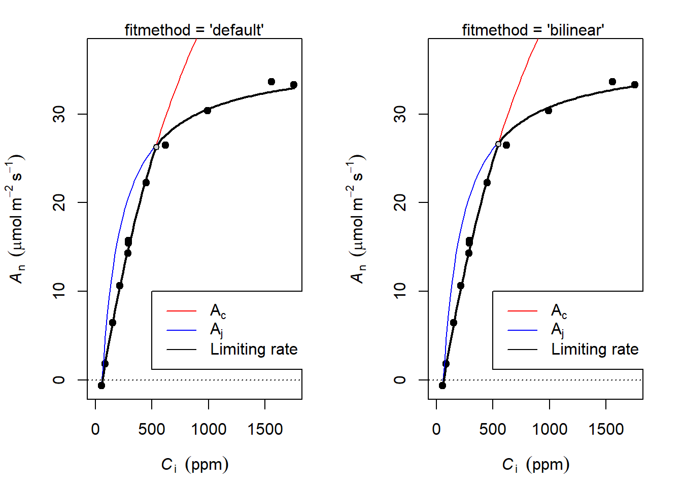

图 3.2: 光合速率的不同的限制阶段

如果需要导出数据做他用，直接根据 attributes 中看到的名称，选择对应的数据导出即可，如果使用 Rstudio 的话，其自动补全的功能在选择数据上更方便。例如导出预测值和系数分别使用如下方式：

# 将模型拟合结果中df（即计算数据）赋给predictaci，
# 并用write.csv导出
predictaci <- acifit$df
write.csv(acifit$df, file = "acipredict.csv")
write.csv(coef(acifit), file = "coefaci.csv")

需要注意的是，因为非线性拟合需要一个初始值，因此，使用默认方式（非线性拟合）的时候，会存在可能的拟合失败现象，此时可以使用 fitmethod = "bilinear"，二者结果略有差别。

3.5.2.1 fitmethod = “onepoint” 介绍

De Kauwe et al. (2016) 发表了关于 one point 方法计算 \(V_{cmax}\) 和 \(J_{max}\) 方法的文章，在 2017 年 11 月的更新中，plantecophys 增加了响应的 R 软件实现方法，该方法并非使用一个点计算 \(V_{cmax}\) 和 \(J_{max}\)，而是对数据集中的每一个点的值进行估计，使用的方法为逆向了光合作用方程。输出为对每个原始数据加入了 \(V_{cmax}\) 和 \(J_{max}\)，当然一如既往的可以使用温度校准的方法。并不建议该方法应用于整个 ACi 曲线的数据，它的假设是在外部环境 CO₂ 浓度和饱和光下，受到 Rubisco 羧化速率的限制而不是 RUBP 的限制。

基于上面的描述，他们的模型如下：

\[\begin{equation} \hat{V}_{cmax} = (A_{sat} + R_{day}) \frac{C_i + K_m}{C_i - \Gamma^*} \tag{3.12} \end{equation}\]

其中：K_m 为米氏常数，其计算为：

\[\begin{equation} K_m = K_c (1 + \frac{O_i}{K_o}) \tag{3.13} \end{equation}\]

未知参数均由文献中的方法进行计算，具体可参考 De Kauwe et al. (2016) 的原文,但上述方法的缺陷为还要使用 ACi 曲线来估算 R_day，因此作者使用了1.5% V_cmax 作为 R_day，因此公式 (3.12) 可变换为：

\[\begin{equation} \hat{V}_{cmax} = A_{sat} (\frac{C_i + K_m}{C_i - \Gamma^*} - 0.015) \tag{3.14} \end{equation}\]

另一个重要的模型的假设为 J_max 与 V_cmax 是成比例的， J_max 的计算是通过 C_i transition point 来实现的，文章中的比值均值为 1.9，范围在 1.68 ~ 2.14 之间。

3.5.3 使用 ‘onepoint’ 单独计算 V_cmax 和 J_max

目前我手头没有相应数据，仅有使用 LI-6400 测试 auto log 2 时的一个数据，我们用这个来示范该方法的使用：

one_data <- read.csv("./data/onepoint.csv")
knitr::kable(head(one_data), booktabs = TRUE,
             caption = 'onepoint 使用的数据')

表 3.2: onepoint 使用的数据
Obs	HHMMSS	FTime	Photo	Cond	Ci	Trmmol	VpdL	CTleaf	Area	BLC_1	StmRat	BLCond	Tair	Tleaf	TBlk	CO2R	CO2S	H2OR	H2OS	RH_R	RH_S	Flow	PARi	PARo	Press	CsMch	HsMch	CsMchSD	HsMchSD	CrMchSD	HrMchSD	StableF	BLCslope	BLCoffst	f_parin	alphaK	Status	fda	Trans	Tair_K	Twall_K	R.W.m2.	Tl.Ta	SVTleaf	h2o_i	h20diff	CTair	SVTair	CndTotal	vp_kPa	VpdA	CndCO2	Ci_Pa	Ci.Ca	RHsfc	C2sfc	AHs.Cs
1	14:12:43	347.0	10.519216	0.1369336	263.0905	1.963046	1.445782	25.89411	6	1.42	1	2.84	25.86572	25.89411	25.86697	412.5374	398.9832	16.98853	19.29724	50.16200	56.97891	500.3231	1198.761	7.497697	98.84273	2.011996	-0.3824501	0.1618589	0.0039255	0.1864786	0.0030409	1.0000000	-0.2195652	2.737392	1	0.16	111115	0.8338718	0.0019630	299.0441	299.0157	191.8018	1.191025	3.353173	33.92433	14.62709	25.87991	3.350355	0.1306349	1.907392	1.442964	0.0821903	26.00458	0.6594024	57.74196	393.9829	0.0154169
2	14:13:04	369.0	10.361122	0.1357092	264.1135	1.946022	1.445559	25.89542	6	1.42	1	2.84	25.86854	25.89542	25.86977	412.5459	399.1890	17.01363	19.30231	50.22723	56.98380	500.3223	1198.748	7.486364	98.84175	2.018435	-0.3787848	0.2174792	0.0025482	0.2455426	0.0025012	1.0000000	-0.2195652	2.737392	1	0.16	111115	0.8338705	0.0019460	299.0454	299.0185	191.7997	1.199722	3.353433	33.92729	14.62498	25.88198	3.350765	0.1295200	1.907874	1.442891	0.0814842	26.10544	0.6616252	57.73418	394.2638	0.0151724
3	14:13:25	373.0	10.207166	0.1342114	264.8348	1.925734	1.445717	25.89660	6	1.42	1	2.84	25.87186	25.89660	25.87317	412.5393	399.3762	17.03833	19.30316	50.29006	56.97489	500.3188	1198.737	7.489428	98.84142	2.018435	-0.3787848	0.2174792	0.0025482	0.2455426	0.0025012	1.0000000	-0.2195652	2.737392	1	0.16	111115	0.8338647	0.0019257	299.0466	299.0219	191.7980	1.210137	3.353668	33.92979	14.62663	25.88423	3.351212	0.1281551	1.907951	1.443261	0.0806199	26.17665	0.6631213	57.71117	394.5242	0.0149311
4	14:13:41	389.5	9.547416	0.1281947	269.6337	1.854272	1.454248	25.94020	6	1.42	1	2.84	25.91845	25.94020	25.92104	413.8090	401.4666	17.12559	19.30638	50.40359	56.82203	500.3162	1199.245	7.449210	98.83208	2.018435	-0.3787848	0.2174792	0.0025482	0.2455426	0.0025012	1.0000000	-0.2195652	2.737392	1	0.16	111115	0.8338604	0.0018543	299.0902	299.0684	191.8792	1.247158	3.362337	34.02071	14.71433	25.92933	3.360173	0.1226580	1.908089	1.452084	0.0771402	26.64846	0.6716216	57.48324	396.9282	0.0138266
5	14:16:16	540.0	10.288968	0.1376602	267.9198	2.009217	1.471788	26.01813	6	1.42	1	2.84	26.01478	26.01813	26.02164	413.9044	400.5999	16.92567	19.28878	49.53554	56.44850	500.3043	1200.785	7.497018	98.81870	2.018435	-0.3787848	0.2174792	0.0025482	0.2455426	0.0025012	0.6666667	-0.2195652	2.737392	1	0.16	111115	0.8338405	0.0020092	299.1681	299.1648	192.1257	1.174669	3.377880	34.18260	14.89382	26.01646	3.377546	0.1312960	1.906093	1.471453	0.0826090	26.47549	0.6687965	57.30143	395.7090	0.0148991
6	14:16:32	555.5	10.178603	0.1381995	269.5898	2.016100	1.471138	26.01657	6	1.42	1	2.84	26.02212	26.01657	26.02939	413.6639	400.4885	16.92345	19.29468	49.49181	56.42595	500.2979	1200.879	7.569045	98.80596	2.018435	-0.3787848	0.2174792	0.0025482	0.2455426	0.0025012	0.6666667	-0.2195652	2.737392	1	0.16	111115	0.8338298	0.0020161	299.1666	299.1721	192.1406	1.172561	3.377567	34.18384	14.88916	26.01934	3.378122	0.1317865	1.906429	1.471693	0.0829197	26.63708	0.6731525	57.32389	395.6501	0.0147473

数据如上所示，为同一个叶片连续记录数据，故所有的光合速率十分接近。

使用方法：

library(plantecophys)

one_data <- subset(one_data, Obs > 0)
one_data$Rd <- 0.5
aci_fit <- fitaci(one_data, fitmethod = "onepoint")

表 3.3: onepoint 法计算的结果
aci_fit.Photo	aci_fit.Vcmax	aci_fit.Jmax
10.519216	47.06893	71.73759
10.361122	46.22091	70.51059
10.207166	45.44617	69.35838
9.547416	41.86217	64.24400
10.288968	45.09335	69.36954
10.178603	44.37360	68.41628

需要注意，为保证结果的精确，如果不设定 Rd, 也即文献中的 Rday，模型是无法计算的，因此上面的示例中虚构了一个，实际操作用一般使用低氧的 ACi 测量计算。

3.5.4 多条 CO₂ 响应曲线的拟合

fitacis 函数实际上是 fitaci 函数的扩展，方便一次拟合多条曲线¹⁰。函数的参数如下：

fitacis(data, group, fitmethod = c("default", 
        "bilinear"),progressbar = TRUE, 
        quiet = FALSE, id = NULL, ...)

## S3 method for class 'acifits'
plot(x, how = c("manyplots", "oneplot"), 
     highlight = NULL, ylim = NULL, 
     xlim = NULL, add = FALSE, what = c("model",
     "data", "none"), ...)

主要参数详解：

实际上 fitacis 与 fitaci 模型算法完全一致，只不过增加了一个 group 参数，用于区分不同测量的数据，具体请参考举例内容。

3.5.4.1 fitacis 函数应用举例

下文代码根据 plantecophys 中的示例代码修改，进行演示，原代码请参考其帮助文档。

library(plantecophys)
# 只提取前10个不同测量的数据，节省时间进行举例
manyacidat2 <- droplevels(manyacidat[manyacidat$Curve %in% 
                                       levels(manyacidat$Curve)[1:10],])

# 对多条曲线进行拟合，使用bilinear方法，
# 仅仅因为其比非线性拟合节省时间
fits <- fitacis(manyacidat2, group = "Curve", fitmethod="bilinear", quiet = TRUE)

# 拟合结果为list，我们可以只提取第一个的拟合结果
fits[[1]]

## Result of fitaci.
## 
## Data and predictions:
##            Ci      Ameas     Amodel         Ac        Aj   Ap        Rd VPD
## 2    53.23129 -0.4401082  0.1014381  0.9601119  2.548123 1000 0.8586158 1.5
## 3    79.47367  2.4824630  2.1937702  3.0526198  7.036734 1000 0.8586158 1.5
## 4   116.74688  5.4531712  4.9419337  5.8011511 11.392394 1000 0.8586158 1.5
## 5   188.00801  9.7099879  9.5705964 10.4310194 16.447715 1000 0.8586158 1.5
## 6   278.44662 14.8225766 14.4261545 15.2897486 19.977583 1000 0.8586158 1.5
## 7   343.03259 17.7982155 17.4602014 18.3289218 21.639847 1000 0.8586158 1.5
## 1   344.72152 17.9244012 17.3165146 18.1849643 21.534276 1000 0.8586158 1.5
## 14  344.74839 16.7933747 17.6853306 18.5545917 21.774261 1000 0.8586158 1.5
## 8   588.08078 23.8925326 24.1309683 27.0327638 25.020148 3000 0.8586158 1.5
## 9   833.25547 26.5674409 25.7783026 33.0856065 26.647921 3000 0.8586158 1.5
## 10 1136.99222 25.9787890 26.8108335 38.1296944 27.676768 3000 0.8586158 1.5
## 11 1436.86370 26.6110657 27.5409345 42.0628463 28.405453 3000 0.8586158 1.5
## 12 1536.46772 27.4018784 27.7965881 43.3773689 28.660781 3000 0.8586158 1.5
## 13 1731.76400 28.6752069 28.0952804 45.2475932 28.959041 3000 0.8586158 1.5
##       Tleaf         Cc     PPFD Patm Ci_original
## 2  24.55873   53.23139 1799.959  100    53.23129
## 3  24.58292   79.47586 1799.590  100    79.47367
## 4  24.71278  116.75183 1799.819  100   116.74688
## 5  24.73687  188.01759 1800.371  100   188.00801
## 6  24.67508  278.46106 1800.233  100   278.44662
## 7  24.76596  343.05006 1799.575  100   343.03259
## 1  24.51593  344.73886 1800.356  100   344.72152
## 14 24.94098  344.76609 1799.964  100   344.74839
## 8  24.83785  588.10494 1799.477  100   588.08078
## 9  24.91185  833.28127 1799.969  100   833.25547
## 10 24.87314 1137.01906 1799.525  100  1136.99222
## 11 24.95914 1436.89126 1799.615  100  1436.86370
## 12 25.04542 1536.49554 1799.784  100  1536.46772
## 13 25.07566 1731.79212 1799.160  100  1731.76400
## 
## Root mean squared error:  2.196037 
## 
## Estimated parameters:
##          Estimate Std. Error
## Vcmax  65.0009909  1.3720635
## Jmax  131.7980133         NA
## Rd      0.8586158  0.2876248
## Note: Vcmax, Jmax are at 25C, Rd is at measurement T.
## 
## Curve was fit using method:  bilinear 
## 
## Parameter settings:
## Patm = 100
##  alpha = 0.24
##  theta = 0.85
##  EaV = 82620.87
##  EdVC = 0
##  delsC = 645.1013
##  EaJ = 39676.89
##  EdVJ = 2e+05
##  delsJ = 641.3615
## 
## Estimated from Tleaf (shown at mean Tleaf):
## GammaStar =  42.31453 
## Km =  698.2084

# 使用sapply提取拟合结果的RMSE(均方根误差)
rmses <- sapply(fits, "[[", "RMSE")
plot(rmses, type='h', ylab="RMSE", xlab="Curve nr")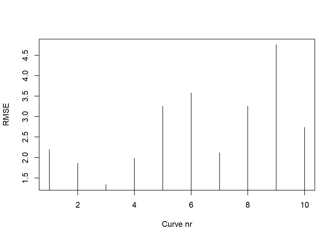

图 3.3: fitacis作图结果

# 对最差的拟合结果进行作图
plot(fits[[which.max(rmses)]])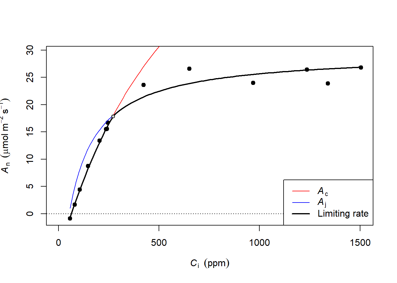

图 3.4: fitacis作图结果

可以看出，fitaci 和 fitacis 用法基本一致，各行代码均已经注释，更详细用法请参函数考帮助。

3.5.5 `findCiTransition` 函数

计算 CiTransition 的函数，第一点为 Ac & Aj，第二点为 Aj & Ap，并且仅在计算 TPU 的前提下才会有第二点出现。

findCiTransition(object, ...)

参数使用，object 为 fitaci 函数对象，或者整个的 Photosyn 函数。 … 为使用 Photosyn 时可传递的参数。

3.6 C4 植物光合

之前的部分模型全部为关于 C3 植物的拟合，而 Caemmerer (2000) 的方法，则是针对 C4 植物的 A-Ci 曲线的实现。

AciC4(Ci, PPFD = 1500, Tleaf = 25, VPMAX25 = 120, 
      JMAX25 = 400, Vcmax = 60, Vpr = 80, 
      alpha = 0, gbs = 0.003, O2 = 210, 
      x = 0.4, THETA = 0.7, Q10 = 2.3, 
      RD0 = 1, RTEMP = 25, TBELOW = 0, 
      DAYRESP = 1, Q10F = 2, FRM = 0.5, ...)

参数详解

Ci：胞间二氧化碳浓度 (\(\mu mol\cdot m^{-2}\cdot s^{-1}\))。
PPFD：光合光量子通量密度 (\(\mu mol\cdot m^{-2}\cdot s^{-1}\))。
Tleaf：叶片温度 ()。
VPMAX25：PEP 羧化最大速率 (\(\mu mol\cdot m^{-2}\cdot s^{-1}\))。
JMAX25：最大电子传递速率 ())。
Vcmax：最大羧化速率(\(\mu mol\cdot m^{-2}\cdot s^{-1}\))。
Vpr：PEP 再生(\(\mu mol\cdot m^{-2}\cdot s^{-1}\))。
alpha：维管束鞘细胞中 PSII 活性的比例。
gbs：维管束鞘导度 (\(mol\cdot m^{-2}\cdot s^{-1}\))。
O2：叶肉细胞氧气浓度。
x：电子传递的分配因子。
THETA：曲角参数。
Q10：Michaelis-Menten 系数中依赖于温度的参数。
RD0：基温下的呼吸 (\(mol\cdot m^{-2}\cdot s^{-1}\))。
RTEMP：呼吸的基温()
TBELOW：此温度以下呼吸为0。
DAYRESP：明呼吸和暗呼吸的比值。
Q10F：呼吸依赖于温度的参数。
FRM：明呼吸中为叶肉呼吸的比例。

以上参数均来自 Caemmerer (2000)，括号中的参数值均为默认值，具体应用时请按照实际情况修改。

3.6.1 C4 植物光合速率的计算

# 模拟 C4 植物的 Ci 值，计算光合速率并作图
library(plantecophys)
aci <- AciC4(Ci=seq(5,600, length=101))
with(aci, plot(Ci, ALEAF, type='l', ylim=c(0,max(ALEAF))))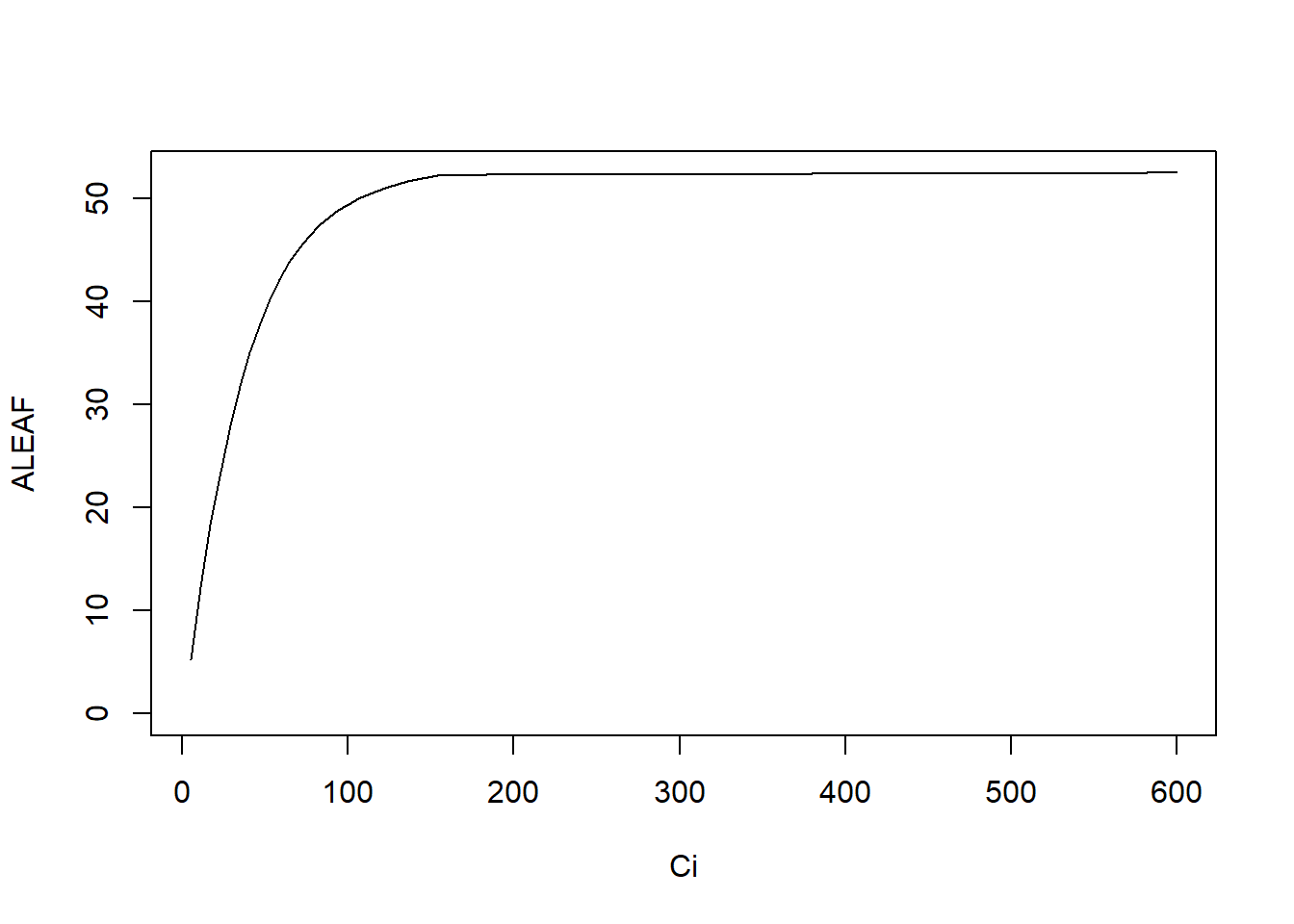

图 3.5: C4 植物 A-Ci 作图

参考文献

Aganchich, B, S Wahbi, F Loreto, and M Centritto. 2009. “Partial Root Zone Drying: Regulation of Photosynthetic Limitations and Antioxidant Enzymatic Activities in Young Olive (Olea Europaea) Saplings.” Tree Physiology 29 (5): 685.

Caemmerer, S. Von. 2000. “Biochemical Models of Leaf Photosynthesis.” Quarterly Review of Biology, 165.

Centritto, M, F Loreto, and K Chartzoulakis. 2003. “The Use of Low Co2 to Estimate Diffusional and Non-Diffusional Limitations of Photosynthetic Capacity of Salt-Stressed Olive Saplings.” Plant Cell and Environment 26 (4): 585–94.

De Kauwe, Martin G, Yan Shih Lin, Ian J Wright, Belinda E Medlyn, Kristine Y Crous, David S Ellsworth, Vincent Maire, I Colin Prentice, Owen K Atkin, and Alistair Rogers. 2016. “A Test of the One Point Method for Estimating Maximum Carboxlation Capacity from Field Measured, Light Saturated Photosynthesis.” New Phytologist 210 (3): 1130.

Duursma, Remko A. 2015. “Plantecophys-an r Package for Analysing and Modelling Leaf Gas Exchange Data.” Plos One 10 (11): e0143346.

Ellsworth, David S, Kristine Y Crous, Hans Lambers, and Julia Cooke. 2015. “Phosphorus Recycling in Photorespiration Maintains High Photosynthetic Capacity in Woody Species.” Plant Cell and Environment 38 (6): 1142–56.

Farquhar, G. D., S. Von Caemmerer, and J. A. Berry. 1980. “A Biochemical Model of Photosynthetic CO\(_2\) Assimilation in Leaves of C3 Species.” Planta 149 (1): 78–90.

Flexas J, Azespejo A, and Berry J A. 2007. “Analysis of Leakage in IRGA’s Leaf Chambers of Open Gas Exchange Systems: Quantification and Its Effects in Photosynthesis Parameterization.” Journal of Experimental Botany 58 (6): 1533.

Gu, Lianhong, Stephen G Pallardy, Kevin Tu, Beverly E Law, and Stan D Wullschleger. 2010. “Reliable Estimation of Biochemical Parameters from c-3 Leaf Photosynthesis-Intercellular Carbon Dioxide Response Curves.” Plant Cell & Environment 33 (11): 1852–74.

Haworth, Matthew, Dilek Killi, Alessandro Materassi, and Antonio Raschi. 2015. “Coordination of Stomatal Physiological Behavior and Morphology with Carbon Dioxide Determines Stomatal Control.” American Journal of Botany 102 (5): 677–88.

Haworth, Matthew, Giovanni Marino, and Mauro Centritto. 2018. “An Introductory Guide to Gas Exchange Analysis of Photosynthesis and Its Application to Plant Phenotyping and Precision Irrigation to Enhance Water Use Efficiency.” Journal of Water and Climate Change. https://doi.org/https://doi.org/10.2166/wcc.2018.152.

Heath, James R, Edward Ayres, Malcolm Possell, Richard D Bardgett, Helaina I J Black, Helen Grant, Phil Ineson, and Gerhard Kerstiens. 2005. “Rising Atmospheric Co2 Reduces Sequestration of Root-Derived Soil Carbon.” Science 309 (5741): 1711–13.

Hikosaka, K, K Ishikawa, A Borjigidai, O Muller, and Y Onoda. 2006. “Temperature Acclimation of Photosynthesis: Mechanisms Involved in the Changes in Temperature Dependence of Photosynthetic Rate.” Journal of Experimental Botany 57 (2): 291.

Lauteri, Marco, Matthew Haworth, Rachid Serraj, Maria Cristina Monteverdi, and Mauro Centritto. 2014. “Photosynthetic Diffusional Constraints Affect Yield in Drought Stressed Rice Cultivars During Flowering.” PLOS ONE 9 (10).

Long, S. P., and C. J. Bernacchi. 2003. “Gas Exchange Measurements, What Can They Tell Us about the Underlying Limitations to Photosynthesis? Procedures and Sources of Error.” Journal of Experimental Botany 54 (392): 2393.

Marshall, B, and P V Biscoe. 1980. “A Model for C3 Leaves Describing the Dependence of Net Photosynthesis on Irradiance.” Journal of Experimental Botany 31 (1): 29–39.

Medlyn, B. E, E Dreyer, D Ellsworth, M Forstreuter, P. C Harley, M. U. F Kirschbaum, X Le Roux, P Montpied, J Strassemeyer, and A Walcroft. 2002. “Temperature Response of Parameters of a Biochemically Based Model of Photosynthesis. II. A Review of Experimental Data Review.” Plant Cell & Environment 25 (9): 1167–79.

Wullschleger, Stan D. 1993. “Biochemical Limitations to Carbon Assimilation in C3 Plants—a Retrospective Analysis of the a-Ci Curves from 109 Species.” Journal of Experimental Botany 44 (262): 907–20.

Yin, Xinyou, P C Struik, Pascual Romero, Jeremy Harbinson, Jochem B Evers, Peter E L Van Der Putten, and J Vos. 2009. “Using Combined Measurements of Gas Exchange and Chlorophyll Fluorescence to Estimate Parameters of a Biochemical C3 Photosynthesis Model: A Critical Appraisal and a New Integrated Approach Applied to Leaves in a Wheat (Triticum Aestivum) Canopy.” Plant Cell and Environment 32 (5): 448–64.

第 3 章 CO2 响应曲线的拟合