第 10 章 LI-6800 的数据分析

10.1 数据格式

此处参考 @ref(batch_question) 相关内容即可。

10.2 LI-6800 与 LI-6400 使用时的差别

plantecophys 使用时建立在 LI-6400XT 基础之上的软件包，因此在 LI-6800 代码中，需要改动的是 fitaci、fitacis 及 fitBB 中的 varnames 选项，也就是将 LI-6400XT 的表头改为 LI-6800 的表头。以 fitaci 函数为例：

 fitaci(aci, varnames = 
        list(ALEAF = "A", Tleaf = "Tleaf", Ci = "Ci", 
          PPFD  = "Qin", Rd = "Rd"))

注：我个人觉得这样使用对于 LI-6800 来讲十分不方便，修改了一下 plantecophys，专门给 LI-6800 使用，具体可参考:

1.使用示例

plantecophys2

10.3 光响应曲线注意事项

光响应曲线的拟合相对简单，仅需要光强和光合速率的值，其中需要修改的部分仅为光强的赋值部分，在文件名一致的前提下，修改如下代码即可：

lrc_Q <- lrc$Qin
lrc_A <- lrc$A

10.4 其他软件包的光响应曲线

FitAQ 软件包

photosynthesis 软件包

10.5 LI-6800 RACiR的测量与拟合

在评估作物性状时，V\(_{cmax}\) 及 J\(_{max}\)时非常有用，传统的 A–Ci 曲线测量要求植物叶片要在一定浓度 CO\(_{2}\) 下适应几分钟后完成测量，这样的测量有几个缺点：

测量时间长，一条曲线至少需要 20 – 30 min，样本量多，重复多时，这种方法几乎没有可行性。
整个测量过程中，时间长，酶的激活状态会有变化，叶绿体会移动，气孔的开度也会发生变化。

而 LI-6800 独有的 auto control 功能在算法上允许用户自定义 CO\(_{2}\) 的起始浓度和种植浓度、变化方式（线性或其他）、所花费的时间，再加上其 IRGAs 极快的响应频率，使得短时间内的 A–Ci 的测量成为现实，即快速 CO\(_{2}\) 响应曲线 RACiR 测量实验，该功能使得 5 min 内测量 A–Ci 曲线成为可能。该方法的实现可参考 J. R. Stinziano et al. (2017) 的文章。

Joseph R. Stinziano et al. (2018) 针对 RACiR技术的疑问做了解答并提出了准确测量的建议，概括如下：

首先，采用 100 ppm/min 的变化速率是与标准方法重合度最高的测量。
其次，明确研究问题，目前已有研究表明Vcmax 与 Jmax 的计算结果与标准测量方法结果无显著差异。
任何条件的改变，都需要做空叶室校准，例如：流速，气体浓度变化方向、温度，斜率等。
空叶室校准与叶片测量采用严格的同一次校准，因为 IRGA 的漂移，需要再次匹配时，或者环境条件改变时，需要重新做空叶室校准。是否需要匹配，可通过不加叶片的最初状态查看，此时 A 值应接近为0，reference 和 sample 气体浓度读数接近相等。
IRGA 分析器使用 5 此多项式进行校准，推荐使用 1 次到 5 次多项式进行拟合，然后根据 BIC 指数来确定最合适的空叶室校准系数（即非参数拟合的模型选择的问题）。确定最合适的浓度变化范围。通常需要去掉最初和最后 30 s的数据。
最小化校准和测量值之间的水分摩尔分数差异。甚至有可能需要控制 reference 或 sample 的水的摩尔分数而不是 Vpdleaf。通过预实验来确定最合适的 \(CO_2\) 变化范围和随时间的斜率。

本文之后关于racir 的空叶室校正部分全部不再支持，因为LI-6800 1.5之后的系统版本，关于两个分析器在快速变化环境条件下的校正均由仪器完成，分析工作直接使用 plantecophys 等软件拟合即可。

例如下面的数据采用了 1.5.02 的 BP 程序 DAT_CO2_Continuous.py，直接测量的 RACiR 数据，结果如下：

remotes::install_github("zhujiedong/plantecophys2")

adyn <- read.csv("data/racir_adyn.csv")

adyn_fit <- plantecophys2::fitaci(adyn)

## Registered S3 methods overwritten by 'plantecophys2':
##   method         from        
##   coef.BBfit     plantecophys
##   coef.BBfits    plantecophys
##   coef.acifit    plantecophys
##   coef.acifits   plantecophys
##   fitted.acifit  plantecophys
##   plot.acifit    plantecophys
##   plot.acifits   plantecophys
##   print.BBfit    plantecophys
##   print.BBfits   plantecophys
##   print.acifit   plantecophys
##   print.acifits  plantecophys
##   summary.acifit plantecophys

## 
## Formula: ALEAF ~ acifun_wrap(Ci, PPFD = PPFD, Vcmax = Vcmax, Jmax = Jmax, 
##     Rd = Rd, Tleaf = Tleaf, Patm = Patm, TcorrectVJ = Tcorrect, 
##     alpha = alpha, theta = theta, gmeso = gmeso, EaV = EaV, EdVC = EdVC, 
##     delsC = delsC, EaJ = EaJ, EdVJ = EdVJ, delsJ = delsJ, Km = Km, 
##     GammaStar = GammaStar)
## 
## Parameters:
##       Estimate Std. Error t value Pr(>|t|)    
## Vcmax 26.99477    0.11547  233.79   <2e-16 ***
## Jmax  46.99725    0.11780  398.96   <2e-16 ***
## Rd     1.38036    0.02146   64.31   <2e-16 ***
## ---
## Signif. codes:  0 '***' 0.001 '**' 0.01 '*' 0.05 '.' 0.1 ' ' 1
## 
## Residual standard error: 0.1347 on 295 degrees of freedom
## 
## Number of iterations to convergence: 7 
## Achieved convergence tolerance: 5.627e-06

plot(adyn_fit)

(#fig:adyn_plot)使用 Adyn 来进行RACiR 的直接测量数据

@ref(fig: dyn_plot) 展示的使用 LI-6800 自带程序测量的数据，无需修正，测量作物为早春温室的水稻。

** 以上为推荐方式，之前的内容自本日（2021.11.12）起正式删除 **

10.6 LI-6800 RACiR簇状叶的测量与拟合

该部分内容请使用 DAT 来测量，实际上后来的 DAT_CO2_Continuous.py 的测量方式参考了这篇文献的内容。代码部分删除，因为新方法无需要再进行校准了。

Coursolle et al. (2019) 测量了簇状叶黑云杉和香脂冷杉两种簇状叶植物的 RACiR，其中的试验方法和结论值得在测量时借鉴，测量方法上：

簇状叶室体积远大于荧光叶室和其他叶室，使用的 \(CO_2\) 的变化为： 15 min 内从 20 ppm 到 1520 ppm 的变化，即变化的速率为 \(100 ppm \cdot min^{-1}\)。但也测试了 200 - 800 ppm的部分曲线。
拟合使用了测量的 Rd，测量方法为：控制 reference 气路在 420 ppm 的 \(CO_2\) 和 22 \(mmol \cdot mol^{-1}\) 的 H₂O 浓度，控制温度为 25 C，诱导后测量 Rd。

得到了一些有帮助的结论：

使用更大的叶室测量 RACiR 是可行的（36 \(cm^2\)），叶室环境的控制需要通过预实验来确定。
该实验使用的 ACi 曲线测量时间在 30 到 36 min，而 RACiR 使用的完整的二氧化碳的浓度范围时，曲线耗时最大的时间接近 22 min。但使用 200 - 800 ppm 范围的变化，则时间可以下降 50%，这些部分范围的测量则可以应用于植物胁迫和表型平台的研究。
实验结果证明只要 match 的调整值保持不变即无需进行空叶室校准（也就是无需匹配的意思，实际的时间间隔取决于仪器的状态），但最新的 range match 功能可有效的增加空叶室校准的时间间隔（新功能，作者试验时尚未推出该功能）。
作者建议最好测量暗呼吸的速率，以获得最佳的 Vcmax 和 Jmax 计算结果。如果有第二台光合仪来测量则可有效的缩短测量时间。

10.7 多个速率的 RACiR 曲线研究

自 RACiR 技术诞生以来，极大的缩短了 Vcmax 以及 Jmax 的测量时间(J. R. Stinziano et al. (2017))，但也引起了一系列争议，作者也对业内的质疑进行了一一的解答 (Joseph R. Stinziano et al. (2018))，但除了因为时间长短导致酶活性，叶绿体位置等差异外，RACiR 还能说明哪些问题呢？Joseph R., Rachael K., and David T. (2019) 最新的研究给出一系列结论：

扩散限制（\(CO_2\) 总导度）和光呼吸导致了表观上的标准 ACi 曲线和 RACiR 测量之间的偏差，表明他们的差异是由生物因子引起，而非仪器导致的人为误差。
上述原因导致的二者之间的偏差，如果不进行修正，那么将显著的低估 \(\Gamma^*\), 除非使用多个速率的 RACiR 来修正。
较高速率的 RACiR 曲线会增大其与标准曲线之间的偏差，但这个差距在无光呼吸的条件下会减小。
因为光呼吸和气体扩散限制与物种相关，结合以上结论，可以使用多个速率的 RACiR 来估算对 \(CO_2\) 的总导度以及相对量的光呼吸速率。

一些可能的方向：

扩散限制影响 Cc 速率的变化，说明对具有较高总阻力与 \(CO_2\) 比值的物种，例如针叶物种，C4 植物，较高的阻力导致 RACiR 与标准 ACi 测量斜率更大的差异，或者测量的前提假设被破坏。
RACiR 可检测到代谢中 \(CO_2\) 的滞后性，各种滞后性的检测对标准 ACi 测量也具有指示性。

文中利用 R 实现了光呼吸之后模型和气体扩散限制模型，本文内容主要对文献中附录材料的源码进行解释：

10.7.1 光呼吸滞后模型

为测试光呼吸的滞后性，作者使用一系列预先设定的参数，模拟了一条 ACc曲线，假定 Rubisco 激活状态为 100%，并且在整个测量过程中气孔导度是不变的。然后使用这些参数来模拟 RACiRs 曲线，并且假定光呼吸分别需要 0, 15, 30, 60, 120 或 300 s 来对变化的 \(CO_2\) 进行响应，在实际效果上，这意味着 Cc 在最初的 0, 15, 30, 60, 120 或 300 内是不变的，最后我们对 \(\Gamma^*\) 和 Ci 使用线性回归进行计算。

10.7.1.1 构造基础数据

模型第一步，则是对需要使用的参数，根据文献和实际情况进行赋值，具体内容参考代码注释。

library(ggplot2)
library(plyr)

## 
## Attaching package: 'plyr'

## The following object is masked from 'package:purrr':
## 
##     compact

library(gridExtra)

# 对图例使用自定义颜色
gg_color_hue <- function(n) {
  hues = seq(15, 375, length = n + 1)
  hcl(h = hues, l = 65, c = 100)[1:n]
}

#Maximum Rubisco carboxylation rate in umol m-2 s-1
Vcmax <- 110

#Maximum Rubisco oxygenation rate in umol m-2 s-1;
#Ratio from Bernacchi et al. 2001. PCE 24:253-259
Vomax <- 0.29 * Vcmax
#Dark respiration in umol m-2 s-1
R <- 2
#Michaelis-Menten constant for Rubisco carboxylation in umol mol-1
Kc <- 404.9
#Michaelis-Menten constant for Rubisco oxygenation in mmol mol-1
Ko <- 278.4
#oxygen concentration in mmol mol-1
O2 <- 210
Kco <- Kc * (1 + O2 / Ko)
#Boundary layer conductance in mol m-2 s-1
BLC <- 2
#stomatal conductance in mol m-2 s-1
gsw <- 0.4
#mesophyll conductance in mol m-2 s-1
gm <- 1
#Chloroplastic CO2 in umol mol-1
Cc <- as.numeric(c(25:400))
#oxygenation rate in umol m-2 s-1
vo <- Vomax * O2 / (O2 + Ko * (1 + Cc / Kc))
#carboxylation rate in umol m-2 s-1
vc <- Vcmax * (Cc) / (Cc + Kco)
#Net CO2 assimilation in umol m-2 s-1
A <- vc - 0.5 * vo - R
#Apparent CO2 assimilation rate in umol m-2 s-1
Aapparent <- vc - 0.5 * vo
#Intercellular CO2 in umol mol-1
Ci <- A / gm + Cc
#Boundary layer CO2 in umol mol-1
Cb <- A / gsw + Ci
#Reference CO2 in umol mol-1
Cr <- A / BLC + Cb

#根据Cc浓度的个数，构造向量
Counter <- as.numeric(c(1:length(Cc)))
#也就是以秒计算的cr与时间的模型
RateCrmodel <- lm(Cr ~ Counter)
#转化为分钟的cr的斜率
RateCr <- coef(RateCrmodel)[2] * 60

#转换为分钟的边界层导度斜率
RateCbmodel <- lm(Cb ~ Counter)
RateCb <- coef(RateCbmodel)[2] * 60

#转换为分钟的ci的斜率
RateCimodel <- lm(Ci ~ Counter)
RateCi <- coef(RateCimodel)[2] * 60

#转换为分钟的Cc的斜率
RateCcmodel <- lm(Cc ~ Counter)
RateCc <- coef(RateCcmodel)[2] * 60

10.7.2 光呼吸滞后性代码

下面代码的目的是为得到 ACi 响应曲线受光呼吸延迟的影响，尤其是在临近补偿点时。

延迟模块

#假定有15s延迟时的数据，即相比上面构造的Cc数据减少15个点
Cc15 <- as.numeric(c((min(Cc) + 15):max(Cc), rep(max(Cc), 15)))
vo15 <- Vomax * O2 / (O2 + Ko * (1 + Cc15 / Kc))
A15 <- vc - 0.5 * vo15 - R
Aapparent15 <- vc - 0.5 * vo15

#30 s 延迟数据
Cc30 <- as.numeric(c((min(Cc) + 30):max(Cc), rep(max(Cc), 30)))
vo30 <- Vomax * O2 / (O2 + Ko * (1 + Cc30 / Kc))
A30 <- vc - 0.5 * vo30 - R
Aapparent30 <- vc - 0.5 * vo30

#60s 延迟数据
Cc60 <- as.numeric(c((min(Cc) + 60):max(Cc), rep(max(Cc), 60)))
vo60 <- Vomax * O2 / (O2 + Ko * (1 + Cc60 / Kc))
A60 <- vc - 0.5 * vo60 - R
Aapparent60 <- vc - 0.5 * vo60

#120s延迟数据
Cc120 <- as.numeric(c((min(Cc) + 120):max(Cc), rep(max(Cc), 120)))
vo120 <- Vomax * O2 / (O2 + Ko * (1 + Cc120 / Kc))
A120 <- vc - 0.5 * vo120 - R
Aapparent120 <- vc - 0.5 * vo120

#300s延迟数据
Cc300 <- as.numeric(c((min(Cc) + 300):max(Cc), rep(max(Cc), 300)))
vo300 <- Vomax * O2 / (O2 + Ko * (1 + Cc300 / Kc))
A300 <- vc - 0.5 * vo120 - R
Aapparent300 <- vc - 0.5 * vo300

10.7.3 数据的构造

下面的代码主要是将上文最终计算的数据构造数据集，并导出。

Anet <- c(A, A15, A30, A60, A120, A300)
Aapp <-
  c(Aapparent,
    Aapparent15,
    Aapparent30,
    Aapparent60,
    Aapparent120,
    Aapparent300)
Ccfull <- rep(Cc, 6)
Cifull <- rep(Ci, 6)
Delay <-
  c(
    rep("0", length(A)),
    rep("15", length(A15)),
    rep("30", length(A30)),
    rep("60", length(A60)),
    rep("120", length(A120)),
    rep("300", length(A300))
  )
PRdata <- as.data.frame(cbind(Anet, Aapp, Ccfull, Cifull, Delay))
write.csv(PRdata, "./data/PRdata.csv")

10.7.4 光呼吸滞后性作图

下面的代码是将光呼吸的数据进行作图。

data <- read.csv("./data/PRdata.csv")
data$Ccfull <- as.numeric(data$Ccfull)
data$Delay <- as.factor(data$Delay)

# 净光合速率与Cc作图
AnetCc <- ggplot(data, aes(x = Ccfull, y = Anet, colour = Delay)) +
  geom_point() +
  labs(x = expression(C[c] ~ "(" * mu * mol ~ mol ^ {
    -1
  } * ")"),
  y = expression(A[net] ~ "(" * mu * mol ~ m ^ {
    -2
  } ~ s ^ {
    -1
  } * ")")) +
  labs(colour = 'Delay (s)') +
  scale_x_continuous(limits = c(25, 100),
                     breaks = c(25, 40, 55, 70, 85, 100)) +
  scale_y_continuous(limits = c(-5, 5)) +
  scale_colour_brewer(palette = 'Spectral') +
  #补偿点的参考线
  geom_hline(yintercept = 0) +
  theme_bw() +
  theme(panel.grid.major = element_blank(),
        panel.grid.minor = element_blank())
AnetCc

## Warning: Removed 1848 rows containing missing values (geom_point).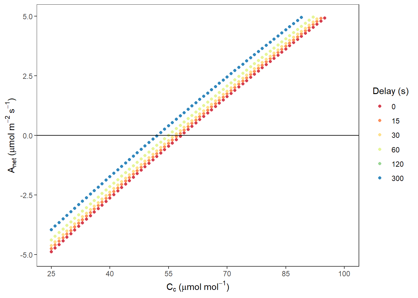

图 10.1: Anet VS. Cc

#净光合速率与Ci作图
AnetCi <- ggplot(data, aes(x = Cifull, y = Anet, colour = Delay)) +
  geom_point() +
  labs(x = expression(C[i] ~ "(" * mu * mol ~ mol ^ {
    -1
  } * ")"),
  y = expression(A[net] ~ "(" * mu * mol ~ m ^ {
    -2
  } ~ s ^ {
    -1
  } * ")")) +
  labs(colour = 'Delay (s)') +
  scale_x_continuous(limits = c(25, 100),
                     breaks = c(25, 40, 55, 70, 85, 100)) +
  scale_y_continuous(limits = c(-5, 5)) +
  scale_colour_brewer(palette = 'Spectral') +
  geom_hline(yintercept = 0) +
  theme_bw() +
  theme(panel.grid.major = element_blank(),
        panel.grid.minor = element_blank())
AnetCi

## Warning: Removed 1878 rows containing missing values (geom_point).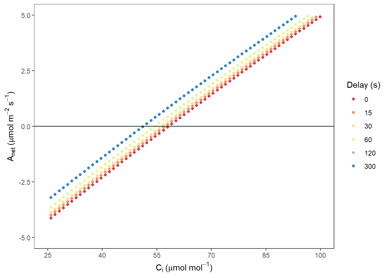

图 10.2: Anet VS. Ci

#表观光合与Cc作图
AappCc <- ggplot(data, aes(x = Ccfull, y = Aapp, colour = Delay)) +
  geom_point() +
  labs(x = expression(C[c] ~ "(" * mu * mol ~ mol ^ {
    -1
  } * ")"),
  y = expression(A[apparent] ~ "(" * mu * mol ~ m ^ {
    -2
  } ~ s ^ {
    -1
  } * ")")) +
  labs(colour = 'Delay (s)') +
  scale_x_continuous(limits = c(25, 75),
                     breaks = c(25, 35, 45, 55, 65, 75)) +
  scale_y_continuous(limits = c(-5, 5)) +
  scale_colour_brewer(palette = 'Spectral') +
  geom_hline(yintercept = 0) +
  theme_bw() +
  theme(panel.grid.major = element_blank(),
        panel.grid.minor = element_blank())
AappCc

## Warning: Removed 1959 rows containing missing values (geom_point).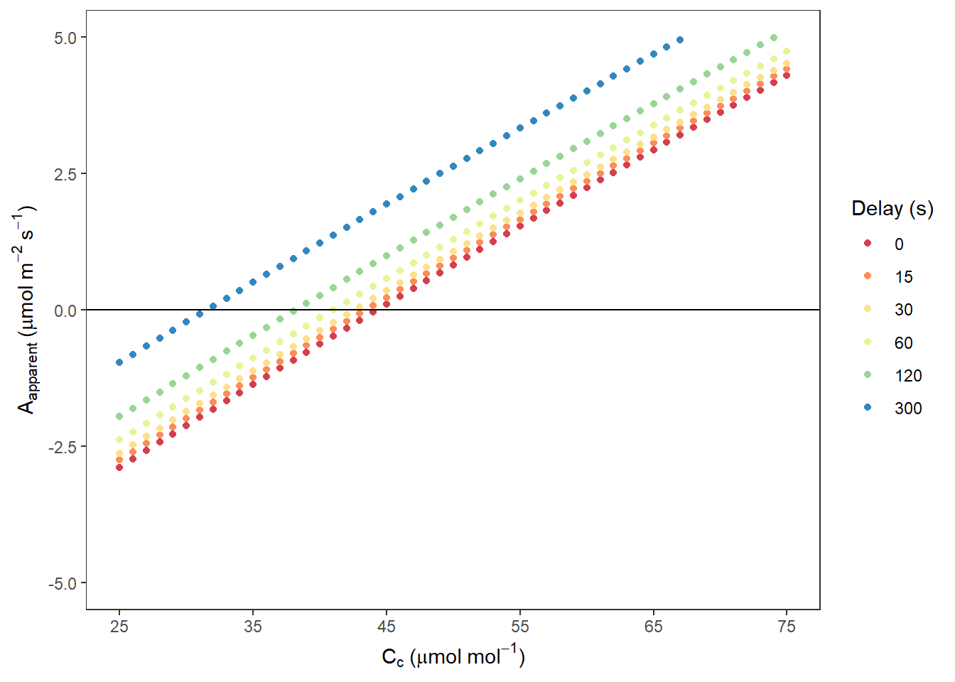

图 10.3: Aapparent VS. Cc

#表观与Ci作图
AappCi <- ggplot(data, aes(x = Cifull, y = Aapp, colour = Delay)) +
  geom_point() +
  labs(x = expression(C[i] ~ "(" * mu * mol ~ mol ^ {
    -1
  } * ")"),
  y = expression(A[apparent] ~ "(" * mu * mol ~ m ^ {
    -2
  } ~ s ^ {
    -1
  } * ")")) +
  labs(colour = 'Delay (s)') +
  scale_x_continuous(limits = c(25, 75),
                     breaks = c(25, 35, 45, 55, 65, 75)) +
  scale_y_continuous(limits = c(-5, 5)) +
  scale_colour_brewer(palette = 'Spectral') +
  geom_hline(yintercept = 0) +
  theme_bw() +
  theme(panel.grid.major = element_blank(),
        panel.grid.minor = element_blank())
AappCi

## Warning: Removed 2003 rows containing missing values (geom_point).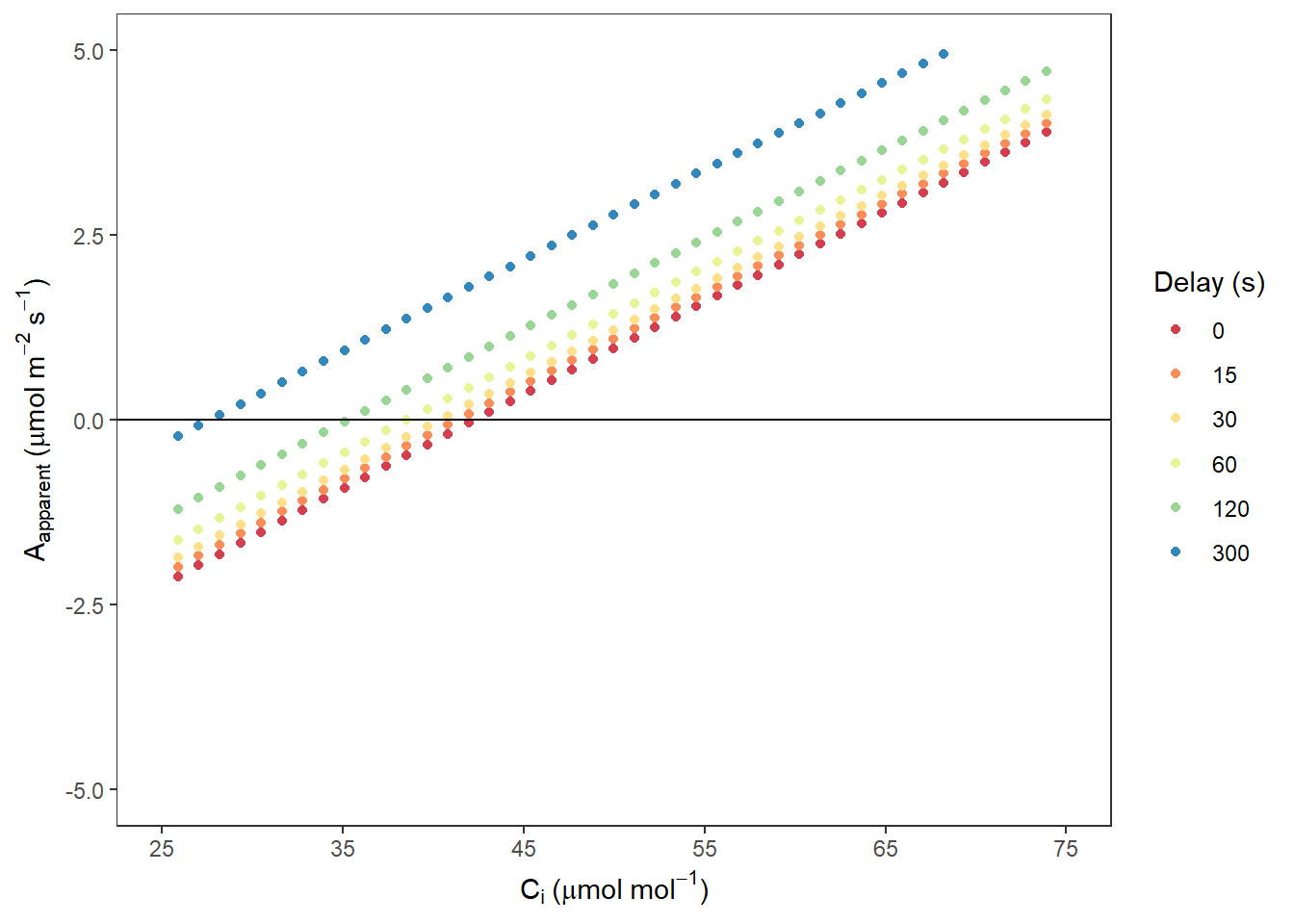

图 10.4: Aapparent VS. Ci

10.7.5 补偿点计算

计算不同的光呼吸时间延迟下的补偿点（基于Ci）：

#对于基于Ci的数据，仅采用ci<100时的数据
dataCi <- data[data$Cifull < 100,]
dataCi0 <- dataCi[dataCi$Delay == "0",]
dataCi15 <- dataCi[dataCi$Delay == "15",]
dataCi30 <- dataCi[dataCi$Delay == "30",]
dataCi60 <- dataCi[dataCi$Delay == "60",]
dataCi120 <- dataCi[dataCi$Delay == "120",]
dataCi300 <- dataCi[dataCi$Delay == "300",]

#光呼吸无延迟时的计算，线性拟合
m1 <- lm(dataCi0$Anet ~ dataCi0$Cifull)
summary(m1)

## 
## Call:
## lm(formula = dataCi0$Anet ~ dataCi0$Cifull)
## 
## Residuals:
##      Min       1Q   Median       3Q      Max 
## -0.13165 -0.04518  0.01711  0.05408  0.06699 
## 
## Coefficients:
##                  Estimate Std. Error t value Pr(>|t|)    
## (Intercept)    -7.2248105  0.0199353  -362.4   <2e-16 ***
## dataCi0$Cifull  0.1228632  0.0003089   397.8   <2e-16 ***
## ---
## Signif. codes:  0 '***' 0.001 '**' 0.01 '*' 0.05 '.' 0.1 ' ' 1
## 
## Residual standard error: 0.06081 on 69 degrees of freedom
## Multiple R-squared:  0.9996, Adjusted R-squared:  0.9996 
## F-statistic: 1.582e+05 on 1 and 69 DF,  p-value: < 2.2e-16

#补偿点为截距比斜率（纵坐标为零）
Gamma0 <- -m1$coefficients[1] / m1$coefficients[2]

#光呼吸延时15s
m2 <- lm(dataCi15$Anet ~ dataCi15$Cifull)
summary(m2)

## 
## Call:
## lm(formula = dataCi15$Anet ~ dataCi15$Cifull)
## 
## Residuals:
##      Min       1Q   Median       3Q      Max 
## -0.13119 -0.04502  0.01705  0.05389  0.06676 
## 
## Coefficients:
##                   Estimate Std. Error t value Pr(>|t|)    
## (Intercept)     -7.0873326  0.0198665  -356.7   <2e-16 ***
## dataCi15$Cifull  0.1225900  0.0003078   398.3   <2e-16 ***
## ---
## Signif. codes:  0 '***' 0.001 '**' 0.01 '*' 0.05 '.' 0.1 ' ' 1
## 
## Residual standard error: 0.0606 on 69 degrees of freedom
## Multiple R-squared:  0.9996, Adjusted R-squared:  0.9996 
## F-statistic: 1.586e+05 on 1 and 69 DF,  p-value: < 2.2e-16

Gamma15 <- -m2$coefficients[1] / m2$coefficients[2]

#光呼吸延时30s
m3 <- lm(dataCi30$Anet ~ dataCi30$Cifull)
summary(m3)

## 
## Call:
## lm(formula = dataCi30$Anet ~ dataCi30$Cifull)
## 
## Residuals:
##      Min       1Q   Median       3Q      Max 
## -0.13076 -0.04488  0.01699  0.05372  0.06654 
## 
## Coefficients:
##                   Estimate Std. Error t value Pr(>|t|)    
## (Intercept)     -6.9553180  0.0198028  -351.2   <2e-16 ***
## dataCi30$Cifull  0.1223321  0.0003068   398.7   <2e-16 ***
## ---
## Signif. codes:  0 '***' 0.001 '**' 0.01 '*' 0.05 '.' 0.1 ' ' 1
## 
## Residual standard error: 0.0604 on 69 degrees of freedom
## Multiple R-squared:  0.9996, Adjusted R-squared:  0.9996 
## F-statistic: 1.59e+05 on 1 and 69 DF,  p-value: < 2.2e-16

Gamma30 <- -m3$coefficients[1] / m3$coefficients[2]

#光呼吸延时60s
m4 <- lm(dataCi60$Anet ~ dataCi60$Cifull)
summary(m4)

## 
## Call:
## lm(formula = dataCi60$Anet ~ dataCi60$Cifull)
## 
## Residuals:
##      Min       1Q   Median       3Q      Max 
## -0.13001 -0.04462  0.01690  0.05341  0.06616 
## 
## Coefficients:
##                  Estimate Std. Error t value Pr(>|t|)    
## (Intercept)     -6.706429   0.019689  -340.6   <2e-16 ***
## dataCi60$Cifull  0.121858   0.000305   399.5   <2e-16 ***
## ---
## Signif. codes:  0 '***' 0.001 '**' 0.01 '*' 0.05 '.' 0.1 ' ' 1
## 
## Residual standard error: 0.06006 on 69 degrees of freedom
## Multiple R-squared:  0.9996, Adjusted R-squared:  0.9996 
## F-statistic: 1.596e+05 on 1 and 69 DF,  p-value: < 2.2e-16

Gamma60 <- -m4$coefficients[1] / m4$coefficients[2]

#光呼吸延时120s
m5 <- lm(dataCi120$Anet ~ dataCi120$Cifull)
summary(m5)

## 
## Call:
## lm(formula = dataCi120$Anet ~ dataCi120$Cifull)
## 
## Residuals:
##      Min       1Q   Median       3Q      Max 
## -0.12879 -0.04421  0.01673  0.05292  0.06555 
## 
## Coefficients:
##                    Estimate Std. Error t value Pr(>|t|)    
## (Intercept)      -6.2616980  0.0195062  -321.0   <2e-16 ***
## dataCi120$Cifull  0.1210486  0.0003022   400.5   <2e-16 ***
## ---
## Signif. codes:  0 '***' 0.001 '**' 0.01 '*' 0.05 '.' 0.1 ' ' 1
## 
## Residual standard error: 0.0595 on 69 degrees of freedom
## Multiple R-squared:  0.9996, Adjusted R-squared:  0.9996 
## F-statistic: 1.604e+05 on 1 and 69 DF,  p-value: < 2.2e-16

Gamma120 <- -m5$coefficients[1] / m5$coefficients[2]

#光呼吸延时300s
m6 <- lm(dataCi300$Anet ~ dataCi300$Cifull)
summary(m6)

## 
## Call:
## lm(formula = dataCi300$Anet ~ dataCi300$Cifull)
## 
## Residuals:
##      Min       1Q   Median       3Q      Max 
## -0.12879 -0.04421  0.01673  0.05292  0.06555 
## 
## Coefficients:
##                    Estimate Std. Error t value Pr(>|t|)    
## (Intercept)      -6.2616980  0.0195062  -321.0   <2e-16 ***
## dataCi300$Cifull  0.1210486  0.0003022   400.5   <2e-16 ***
## ---
## Signif. codes:  0 '***' 0.001 '**' 0.01 '*' 0.05 '.' 0.1 ' ' 1
## 
## Residual standard error: 0.0595 on 69 degrees of freedom
## Multiple R-squared:  0.9996, Adjusted R-squared:  0.9996 
## F-statistic: 1.604e+05 on 1 and 69 DF,  p-value: < 2.2e-16

Gamma300 <- -m6$coefficients[1] / m6$coefficients[2]

构造数据并作图

GammaCi <- c(Gamma0, Gamma15, Gamma30, Gamma60, Gamma120, Gamma300)

ints <-
  c(
    m1$coefficients[1],
    m2$coefficients[1],
    m3$coefficients[1],
    m4$coefficients[1],
    m5$coefficients[1],
    m6$coefficients[1]
  )
slps <-
  c(
    0,
    m2$coefficients[2] - m1$coefficients[2],
    m3$coefficients[2] - m1$coefficients[2],
    m4$coefficients[2] - m1$coefficients[2],
    m5$coefficients[2] - m1$coefficients[2],
    m6$coefficients[2] - m1$coefficients[2]
  )
dels <- c(0, 15, 30, 60, 120, 300)
summary(lm(ints ~ dels))

## 
## Call:
## lm(formula = ints ~ dels)
## 
## Residuals:
##   (Intercept) (Intercept).1 (Intercept).2 (Intercept).3 (Intercept).4 
##      -0.20351      -0.11262      -0.02719       0.12853       0.38691 
## (Intercept).5 
##      -0.17212 
## 
## Coefficients:
##               Estimate Std. Error t value Pr(>|t|)    
## (Intercept) -7.0213001  0.1343090 -52.277 8.01e-07 ***
## dels         0.0031057  0.0009959   3.119   0.0356 *  
## ---
## Signif. codes:  0 '***' 0.001 '**' 0.01 '*' 0.05 '.' 0.1 ' ' 1
## 
## Residual standard error: 0.2503 on 4 degrees of freedom
## Multiple R-squared:  0.7086, Adjusted R-squared:  0.6357 
## F-statistic: 9.725 on 1 and 4 DF,  p-value: 0.03558

plot(ints ~ dels)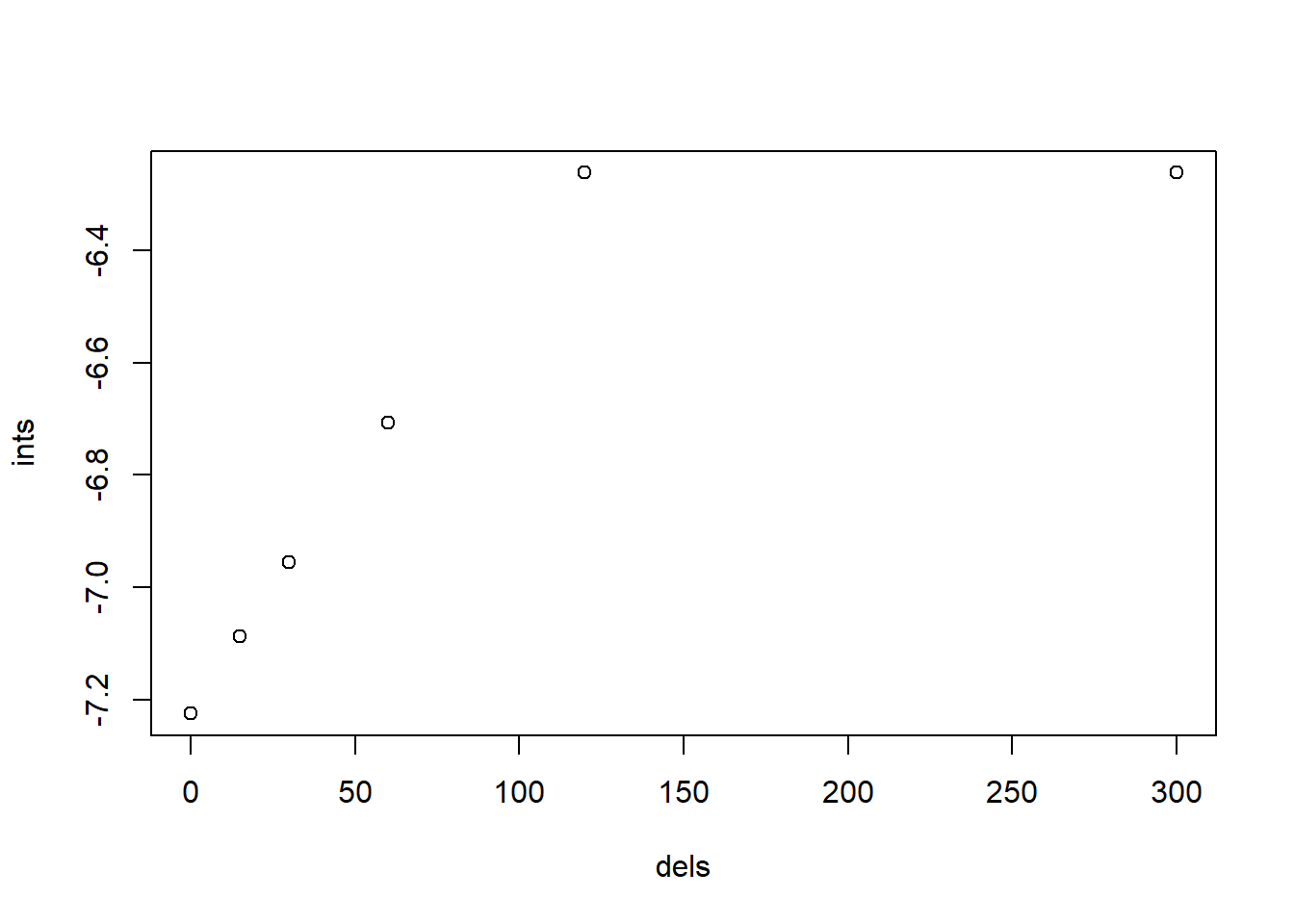

图 10.5: 基于 Ci 的不同延时下的截距

plot(slps ~ dels)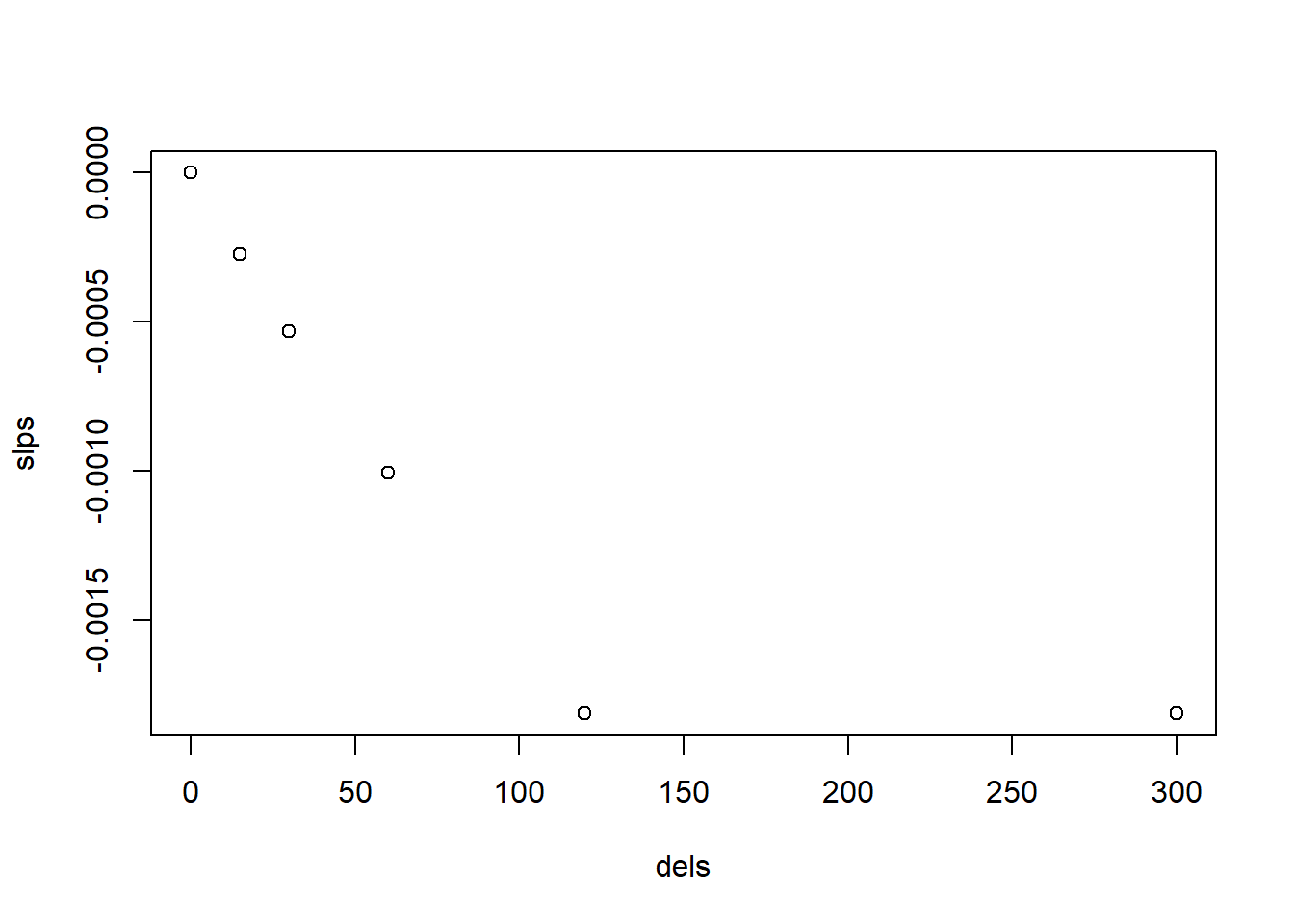

图 10.6: 基于 Ci 的不同延时下的斜率变化

summary(lm(slps ~ dels - 1))

## 
## Call:
## lm(formula = slps ~ dels - 1)
## 
## Residuals:
##                   dataCi15$Cifull  dataCi30$Cifull  dataCi60$Cifull 
##       -2.711e-19       -1.574e-04       -2.995e-04       -5.424e-04 
## dataCi120$Cifull dataCi300$Cifull 
##       -8.881e-04        5.015e-04 
## 
## Coefficients:
##       Estimate Std. Error t value Pr(>|t|)   
## dels -7.72e-06   1.63e-06  -4.738  0.00516 **
## ---
## Signif. codes:  0 '***' 0.001 '**' 0.01 '*' 0.05 '.' 0.1 ' ' 1
## 
## Residual standard error: 0.0005383 on 5 degrees of freedom
## Multiple R-squared:  0.8178, Adjusted R-squared:  0.7814 
## F-statistic: 22.44 on 1 and 5 DF,  p-value: 0.005161

基于 Cc 的补偿点计算结果:

# 仅使用 Cc < 75的数据点拟合，过程同ci
dataCc <- data[data$Ccfull < 75, ]
dataCc0 <- dataCc[dataCc$Delay == "0", ]
dataCc15 <- dataCc[dataCc$Delay == "15", ]
dataCc30 <- dataCc[dataCc$Delay == "30", ]
dataCc60 <- dataCc[dataCc$Delay == "60", ]
dataCc120 <- dataCc[dataCc$Delay == "120", ]
dataCc300 <- dataCc[dataCc$Delay == "300", ]

# 无延迟数据
m1 <- lm(dataCc0$Anet ~ dataCc0$Ccfull)
summary(m1)

## 
## Call:
## lm(formula = dataCc0$Anet ~ dataCc0$Ccfull)
## 
## Residuals:
##       Min        1Q    Median        3Q       Max 
## -0.075648 -0.025444  0.009857  0.031706  0.039431 
## 
## Coefficients:
##                  Estimate Std. Error t value Pr(>|t|)    
## (Intercept)    -8.4062011  0.0181852  -462.3   <2e-16 ***
## dataCc0$Ccfull  0.1438710  0.0003527   407.9   <2e-16 ***
## ---
## Signif. codes:  0 '***' 0.001 '**' 0.01 '*' 0.05 '.' 0.1 ' ' 1
## 
## Residual standard error: 0.03599 on 48 degrees of freedom
## Multiple R-squared:  0.9997, Adjusted R-squared:  0.9997 
## F-statistic: 1.664e+05 on 1 and 48 DF,  p-value: < 2.2e-16

Gamma0 <- -m1$coefficients[1] / m1$coefficients[2]

#延时15s数据
m2 <- lm(dataCc15$Anet ~ dataCc15$Ccfull)
summary(m2)

## 
## Call:
## lm(formula = dataCc15$Anet ~ dataCc15$Ccfull)
## 
## Residuals:
##       Min        1Q    Median        3Q       Max 
## -0.075393 -0.025359  0.009824  0.031599  0.039299 
## 
## Coefficients:
##                   Estimate Std. Error t value Pr(>|t|)    
## (Intercept)     -8.2659145  0.0181243  -456.1   <2e-16 ***
## dataCc15$Ccfull  0.1435470  0.0003515   408.4   <2e-16 ***
## ---
## Signif. codes:  0 '***' 0.001 '**' 0.01 '*' 0.05 '.' 0.1 ' ' 1
## 
## Residual standard error: 0.03587 on 48 degrees of freedom
## Multiple R-squared:  0.9997, Adjusted R-squared:  0.9997 
## F-statistic: 1.668e+05 on 1 and 48 DF,  p-value: < 2.2e-16

Gamma15 <- -m2$coefficients[1] / m2$coefficients[2]

#延时30s数据
m3 <- lm(dataCc30$Anet ~ dataCc30$Ccfull)
summary(m3)

## 
## Call:
## lm(formula = dataCc30$Anet ~ dataCc30$Ccfull)
## 
## Residuals:
##       Min        1Q    Median        3Q       Max 
## -0.075158 -0.025280  0.009794  0.031501  0.039177 
## 
## Coefficients:
##                   Estimate Std. Error t value Pr(>|t|)    
## (Intercept)     -8.1312578  0.0180681  -450.0   <2e-16 ***
## dataCc30$Ccfull  0.1432414  0.0003504   408.8   <2e-16 ***
## ---
## Signif. codes:  0 '***' 0.001 '**' 0.01 '*' 0.05 '.' 0.1 ' ' 1
## 
## Residual standard error: 0.03576 on 48 degrees of freedom
## Multiple R-squared:  0.9997, Adjusted R-squared:  0.9997 
## F-statistic: 1.671e+05 on 1 and 48 DF,  p-value: < 2.2e-16

Gamma30 <- -m3$coefficients[1] / m3$coefficients[2]

#延时60s数据
m4 <- lm(dataCc60$Anet ~ dataCc60$Ccfull)
summary(m4)

## 
## Call:
## lm(formula = dataCc60$Anet ~ dataCc60$Ccfull)
## 
## Residuals:
##       Min        1Q    Median        3Q       Max 
## -0.074737 -0.025139  0.009739  0.031325  0.038959 
## 
## Coefficients:
##                   Estimate Std. Error t value Pr(>|t|)    
## (Intercept)     -7.8775340  0.0179675  -438.4   <2e-16 ***
## dataCc60$Ccfull  0.1426797  0.0003485   409.4   <2e-16 ***
## ---
## Signif. codes:  0 '***' 0.001 '**' 0.01 '*' 0.05 '.' 0.1 ' ' 1
## 
## Residual standard error: 0.03556 on 48 degrees of freedom
## Multiple R-squared:  0.9997, Adjusted R-squared:  0.9997 
## F-statistic: 1.676e+05 on 1 and 48 DF,  p-value: < 2.2e-16

Gamma60 <- -m4$coefficients[1] / m4$coefficients[2]

#延时120s数据
m5 <- lm(dataCc120$Anet ~ dataCc120$Ccfull)
summary(m5)

## 
## Call:
## lm(formula = dataCc120$Anet ~ dataCc120$Ccfull)
## 
## Residuals:
##       Min        1Q    Median        3Q       Max 
## -0.074060 -0.024912  0.009651  0.031042  0.038607 
## 
## Coefficients:
##                    Estimate Std. Error t value Pr(>|t|)    
## (Intercept)      -7.4246412  0.0178052  -417.0   <2e-16 ***
## dataCc120$Ccfull  0.1417238  0.0003453   410.4   <2e-16 ***
## ---
## Signif. codes:  0 '***' 0.001 '**' 0.01 '*' 0.05 '.' 0.1 ' ' 1
## 
## Residual standard error: 0.03524 on 48 degrees of freedom
## Multiple R-squared:  0.9997, Adjusted R-squared:  0.9997 
## F-statistic: 1.684e+05 on 1 and 48 DF,  p-value: < 2.2e-16

Gamma120 <- -m5$coefficients[1] / m5$coefficients[2]

#延时300s数据
m6 <- lm(dataCc300$Anet ~ dataCc300$Ccfull)
summary(m6)

## 
## Call:
## lm(formula = dataCc300$Anet ~ dataCc300$Ccfull)
## 
## Residuals:
##       Min        1Q    Median        3Q       Max 
## -0.074060 -0.024912  0.009651  0.031042  0.038607 
## 
## Coefficients:
##                    Estimate Std. Error t value Pr(>|t|)    
## (Intercept)      -7.4246412  0.0178052  -417.0   <2e-16 ***
## dataCc300$Ccfull  0.1417238  0.0003453   410.4   <2e-16 ***
## ---
## Signif. codes:  0 '***' 0.001 '**' 0.01 '*' 0.05 '.' 0.1 ' ' 1
## 
## Residual standard error: 0.03524 on 48 degrees of freedom
## Multiple R-squared:  0.9997, Adjusted R-squared:  0.9997 
## F-statistic: 1.684e+05 on 1 and 48 DF,  p-value: < 2.2e-16

Gamma300 <- -m6$coefficients[1] / m6$coefficients[2]

GammaCc <- c(Gamma0, Gamma15, Gamma30, Gamma60, Gamma120, Gamma300)

ints <-
  c(
    m1$coefficients[1],
    m2$coefficients[1],
    m3$coefficients[1],
    m4$coefficients[1],
    m5$coefficients[1],
    m6$coefficients[1]
  )
dels <- c(0, 15, 30, 60, 120, 300)
plot(ints ~ dels)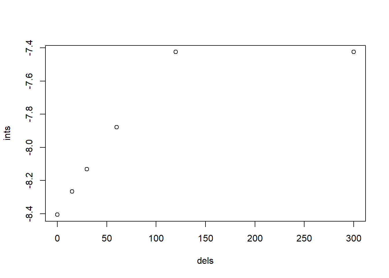

图 10.7: 基于 Cc 的不同延时下的时间

summary(lm(ints ~ dels))

## 
## Call:
## lm(formula = ints ~ dels)
## 
## Residuals:
##   (Intercept) (Intercept).1 (Intercept).2 (Intercept).3 (Intercept).4 
##      -0.20760      -0.11478      -0.02759       0.13119       0.39421 
## (Intercept).5 
##      -0.17542 
## 
## Coefficients:
##              Estimate Std. Error t value Pr(>|t|)    
## (Intercept) -8.198602   0.136891 -59.891 4.65e-07 ***
## dels         0.003165   0.001015   3.118   0.0356 *  
## ---
## Signif. codes:  0 '***' 0.001 '**' 0.01 '*' 0.05 '.' 0.1 ' ' 1
## 
## Residual standard error: 0.2552 on 4 degrees of freedom
## Multiple R-squared:  0.7085, Adjusted R-squared:  0.6356 
## F-statistic:  9.72 on 1 and 4 DF,  p-value: 0.03561

#GammaStar
# For Ci-based estimates, only use Ci < 100
dataCi <- data[data$Cifull < 100,]
dataCi0 <- dataCi[dataCi$Delay == "0",]
dataCi15 <- dataCi[dataCi$Delay == "15",]
dataCi30 <- dataCi[dataCi$Delay == "30",]
dataCi60 <- dataCi[dataCi$Delay == "60",]
dataCi120 <- dataCi[dataCi$Delay == "120",]
dataCi300 <- dataCi[dataCi$Delay == "300",]
m1 <- lm(dataCi0$Aapp ~ dataCi0$Cifull)
summary(m1)

## 
## Call:
## lm(formula = dataCi0$Aapp ~ dataCi0$Cifull)
## 
## Residuals:
##      Min       1Q   Median       3Q      Max 
## -0.13165 -0.04518  0.01711  0.05408  0.06699 
## 
## Coefficients:
##                  Estimate Std. Error t value Pr(>|t|)    
## (Intercept)    -5.2248105  0.0199353  -262.1   <2e-16 ***
## dataCi0$Cifull  0.1228632  0.0003089   397.8   <2e-16 ***
## ---
## Signif. codes:  0 '***' 0.001 '**' 0.01 '*' 0.05 '.' 0.1 ' ' 1
## 
## Residual standard error: 0.06081 on 69 degrees of freedom
## Multiple R-squared:  0.9996, Adjusted R-squared:  0.9996 
## F-statistic: 1.582e+05 on 1 and 69 DF,  p-value: < 2.2e-16

Gamma0 <- -m1$coefficients[1] / m1$coefficients[2]
m2 <- lm(dataCi15$Aapp ~ dataCi15$Cifull)
summary(m2)

## 
## Call:
## lm(formula = dataCi15$Aapp ~ dataCi15$Cifull)
## 
## Residuals:
##      Min       1Q   Median       3Q      Max 
## -0.13119 -0.04502  0.01705  0.05389  0.06676 
## 
## Coefficients:
##                   Estimate Std. Error t value Pr(>|t|)    
## (Intercept)     -5.0873326  0.0198665  -256.1   <2e-16 ***
## dataCi15$Cifull  0.1225900  0.0003078   398.3   <2e-16 ***
## ---
## Signif. codes:  0 '***' 0.001 '**' 0.01 '*' 0.05 '.' 0.1 ' ' 1
## 
## Residual standard error: 0.0606 on 69 degrees of freedom
## Multiple R-squared:  0.9996, Adjusted R-squared:  0.9996 
## F-statistic: 1.586e+05 on 1 and 69 DF,  p-value: < 2.2e-16

Gamma15 <- -m2$coefficients[1] / m2$coefficients[2]
m3 <- lm(dataCi30$Aapp ~ dataCi30$Cifull)
summary(m3)

## 
## Call:
## lm(formula = dataCi30$Aapp ~ dataCi30$Cifull)
## 
## Residuals:
##      Min       1Q   Median       3Q      Max 
## -0.13076 -0.04488  0.01699  0.05372  0.06654 
## 
## Coefficients:
##                   Estimate Std. Error t value Pr(>|t|)    
## (Intercept)     -4.9553180  0.0198028  -250.2   <2e-16 ***
## dataCi30$Cifull  0.1223321  0.0003068   398.7   <2e-16 ***
## ---
## Signif. codes:  0 '***' 0.001 '**' 0.01 '*' 0.05 '.' 0.1 ' ' 1
## 
## Residual standard error: 0.0604 on 69 degrees of freedom
## Multiple R-squared:  0.9996, Adjusted R-squared:  0.9996 
## F-statistic: 1.59e+05 on 1 and 69 DF,  p-value: < 2.2e-16

Gamma30 <- -m3$coefficients[1] / m3$coefficients[2]
m4 <- lm(dataCi60$Aapp ~ dataCi60$Cifull)
summary(m4)

## 
## Call:
## lm(formula = dataCi60$Aapp ~ dataCi60$Cifull)
## 
## Residuals:
##      Min       1Q   Median       3Q      Max 
## -0.13001 -0.04462  0.01690  0.05341  0.06616 
## 
## Coefficients:
##                  Estimate Std. Error t value Pr(>|t|)    
## (Intercept)     -4.706429   0.019689  -239.0   <2e-16 ***
## dataCi60$Cifull  0.121858   0.000305   399.5   <2e-16 ***
## ---
## Signif. codes:  0 '***' 0.001 '**' 0.01 '*' 0.05 '.' 0.1 ' ' 1
## 
## Residual standard error: 0.06006 on 69 degrees of freedom
## Multiple R-squared:  0.9996, Adjusted R-squared:  0.9996 
## F-statistic: 1.596e+05 on 1 and 69 DF,  p-value: < 2.2e-16

Gamma60 <- -m4$coefficients[1] / m4$coefficients[2]
m5 <- lm(dataCi120$Aapp ~ dataCi120$Cifull)
summary(m5)

## 
## Call:
## lm(formula = dataCi120$Aapp ~ dataCi120$Cifull)
## 
## Residuals:
##      Min       1Q   Median       3Q      Max 
## -0.12879 -0.04421  0.01673  0.05292  0.06555 
## 
## Coefficients:
##                    Estimate Std. Error t value Pr(>|t|)    
## (Intercept)      -4.2616980  0.0195062  -218.5   <2e-16 ***
## dataCi120$Cifull  0.1210486  0.0003022   400.5   <2e-16 ***
## ---
## Signif. codes:  0 '***' 0.001 '**' 0.01 '*' 0.05 '.' 0.1 ' ' 1
## 
## Residual standard error: 0.0595 on 69 degrees of freedom
## Multiple R-squared:  0.9996, Adjusted R-squared:  0.9996 
## F-statistic: 1.604e+05 on 1 and 69 DF,  p-value: < 2.2e-16

Gamma120 <- -m5$coefficients[1] / m5$coefficients[2]
m6 <- lm(dataCi300$Aapp ~ dataCi300$Cifull)
summary(m6)

## 
## Call:
## lm(formula = dataCi300$Aapp ~ dataCi300$Cifull)
## 
## Residuals:
##      Min       1Q   Median       3Q      Max 
## -0.12662 -0.04346  0.01645  0.05202  0.06444 
## 
## Coefficients:
##                    Estimate Std. Error t value Pr(>|t|)    
## (Intercept)      -3.2402030  0.0191773  -169.0   <2e-16 ***
## dataCi300$Cifull  0.1193852  0.0002971   401.8   <2e-16 ***
## ---
## Signif. codes:  0 '***' 0.001 '**' 0.01 '*' 0.05 '.' 0.1 ' ' 1
## 
## Residual standard error: 0.05849 on 69 degrees of freedom
## Multiple R-squared:  0.9996, Adjusted R-squared:  0.9996 
## F-statistic: 1.615e+05 on 1 and 69 DF,  p-value: < 2.2e-16

Gamma300 <- -m6$coefficients[1] / m6$coefficients[2]

GammastarCi <-
  c(Gamma0, Gamma15, Gamma30, Gamma60, Gamma120, Gamma300)

# For Cc-based estimates, only use Cc < 75
dataCc <- data[data$Ccfull < 75,]
dataCc0 <- dataCc[dataCc$Delay == "0",]
dataCc15 <- dataCc[dataCc$Delay == "15",]
dataCc30 <- dataCc[dataCc$Delay == "30",]
dataCc60 <- dataCc[dataCc$Delay == "60",]
dataCc120 <- dataCc[dataCc$Delay == "120",]
dataCc300 <- dataCc[dataCc$Delay == "300",]
m1 <- lm(dataCc0$Aapp ~ dataCc0$Ccfull)
summary(m1)

## 
## Call:
## lm(formula = dataCc0$Aapp ~ dataCc0$Ccfull)
## 
## Residuals:
##       Min        1Q    Median        3Q       Max 
## -0.075648 -0.025444  0.009857  0.031706  0.039431 
## 
## Coefficients:
##                  Estimate Std. Error t value Pr(>|t|)    
## (Intercept)    -6.4062011  0.0181852  -352.3   <2e-16 ***
## dataCc0$Ccfull  0.1438710  0.0003527   407.9   <2e-16 ***
## ---
## Signif. codes:  0 '***' 0.001 '**' 0.01 '*' 0.05 '.' 0.1 ' ' 1
## 
## Residual standard error: 0.03599 on 48 degrees of freedom
## Multiple R-squared:  0.9997, Adjusted R-squared:  0.9997 
## F-statistic: 1.664e+05 on 1 and 48 DF,  p-value: < 2.2e-16

Gamma0 <- -m1$coefficients[1] / m1$coefficients[2]
m2 <- lm(dataCc15$Aapp ~ dataCc15$Ccfull)
summary(m2)

## 
## Call:
## lm(formula = dataCc15$Aapp ~ dataCc15$Ccfull)
## 
## Residuals:
##       Min        1Q    Median        3Q       Max 
## -0.075393 -0.025359  0.009824  0.031599  0.039299 
## 
## Coefficients:
##                   Estimate Std. Error t value Pr(>|t|)    
## (Intercept)     -6.2659145  0.0181243  -345.7   <2e-16 ***
## dataCc15$Ccfull  0.1435470  0.0003515   408.4   <2e-16 ***
## ---
## Signif. codes:  0 '***' 0.001 '**' 0.01 '*' 0.05 '.' 0.1 ' ' 1
## 
## Residual standard error: 0.03587 on 48 degrees of freedom
## Multiple R-squared:  0.9997, Adjusted R-squared:  0.9997 
## F-statistic: 1.668e+05 on 1 and 48 DF,  p-value: < 2.2e-16

Gamma15 <- -m2$coefficients[1] / m2$coefficients[2]
m3 <- lm(dataCc30$Aapp ~ dataCc30$Ccfull)
summary(m3)

## 
## Call:
## lm(formula = dataCc30$Aapp ~ dataCc30$Ccfull)
## 
## Residuals:
##       Min        1Q    Median        3Q       Max 
## -0.075158 -0.025280  0.009794  0.031501  0.039177 
## 
## Coefficients:
##                   Estimate Std. Error t value Pr(>|t|)    
## (Intercept)     -6.1312578  0.0180681  -339.3   <2e-16 ***
## dataCc30$Ccfull  0.1432414  0.0003504   408.8   <2e-16 ***
## ---
## Signif. codes:  0 '***' 0.001 '**' 0.01 '*' 0.05 '.' 0.1 ' ' 1
## 
## Residual standard error: 0.03576 on 48 degrees of freedom
## Multiple R-squared:  0.9997, Adjusted R-squared:  0.9997 
## F-statistic: 1.671e+05 on 1 and 48 DF,  p-value: < 2.2e-16

Gamma30 <- -m3$coefficients[1] / m3$coefficients[2]
m4 <- lm(dataCc60$Aapp ~ dataCc60$Ccfull)
summary(m4)

## 
## Call:
## lm(formula = dataCc60$Aapp ~ dataCc60$Ccfull)
## 
## Residuals:
##       Min        1Q    Median        3Q       Max 
## -0.074737 -0.025139  0.009739  0.031325  0.038959 
## 
## Coefficients:
##                   Estimate Std. Error t value Pr(>|t|)    
## (Intercept)     -5.8775340  0.0179675  -327.1   <2e-16 ***
## dataCc60$Ccfull  0.1426797  0.0003485   409.4   <2e-16 ***
## ---
## Signif. codes:  0 '***' 0.001 '**' 0.01 '*' 0.05 '.' 0.1 ' ' 1
## 
## Residual standard error: 0.03556 on 48 degrees of freedom
## Multiple R-squared:  0.9997, Adjusted R-squared:  0.9997 
## F-statistic: 1.676e+05 on 1 and 48 DF,  p-value: < 2.2e-16

Gamma60 <- -m4$coefficients[1] / m4$coefficients[2]
m5 <- lm(dataCc120$Aapp ~ dataCc120$Ccfull)
summary(m5)

## 
## Call:
## lm(formula = dataCc120$Aapp ~ dataCc120$Ccfull)
## 
## Residuals:
##       Min        1Q    Median        3Q       Max 
## -0.074060 -0.024912  0.009651  0.031042  0.038607 
## 
## Coefficients:
##                    Estimate Std. Error t value Pr(>|t|)    
## (Intercept)      -5.4246412  0.0178052  -304.7   <2e-16 ***
## dataCc120$Ccfull  0.1417238  0.0003453   410.4   <2e-16 ***
## ---
## Signif. codes:  0 '***' 0.001 '**' 0.01 '*' 0.05 '.' 0.1 ' ' 1
## 
## Residual standard error: 0.03524 on 48 degrees of freedom
## Multiple R-squared:  0.9997, Adjusted R-squared:  0.9997 
## F-statistic: 1.684e+05 on 1 and 48 DF,  p-value: < 2.2e-16

Gamma120 <- -m5$coefficients[1] / m5$coefficients[2]
m6 <- lm(dataCc300$Aapp ~ dataCc300$Ccfull)
summary(m6)

## 
## Call:
## lm(formula = dataCc300$Aapp ~ dataCc300$Ccfull)
## 
## Residuals:
##       Min        1Q    Median        3Q       Max 
## -0.072835 -0.024500  0.009492  0.030529  0.037969 
## 
## Coefficients:
##                    Estimate Std. Error t value Pr(>|t|)    
## (Intercept)      -4.3867121  0.0175110  -250.5   <2e-16 ***
## dataCc300$Ccfull  0.1397661  0.0003396   411.5   <2e-16 ***
## ---
## Signif. codes:  0 '***' 0.001 '**' 0.01 '*' 0.05 '.' 0.1 ' ' 1
## 
## Residual standard error: 0.03466 on 48 degrees of freedom
## Multiple R-squared:  0.9997, Adjusted R-squared:  0.9997 
## F-statistic: 1.694e+05 on 1 and 48 DF,  p-value: < 2.2e-16

Gamma300 <- -m6$coefficients[1] / m6$coefficients[2]

GammastarCc <-
  c(Gamma0, Gamma15, Gamma30, Gamma60, Gamma120, Gamma300)

Delay2 <- c("0", "15", "30", "60", "120", "300")
PRcomps <-
  as.data.frame(cbind(Delay2, GammaCc, GammaCi, GammastarCc, GammastarCi))
write.csv(PRcomps, "./data/PRcomps.csv")

ints <-
  c(
    m1$coefficients[1],
    m2$coefficients[1],
    m3$coefficients[1],
    m4$coefficients[1],
    m5$coefficients[1],
    m6$coefficients[1]
  )
dels <- c(0, 15, 30, 60, 120, 300)
summary(lm(ints ~ dels))

## 
## Call:
## lm(formula = ints ~ dels)
## 
## Residuals:
##   (Intercept) (Intercept).1 (Intercept).2 (Intercept).3 (Intercept).4 
##    -0.0751633    -0.0347043     0.0001247     0.0541933     0.1077758 
## (Intercept).5 
##    -0.0522262 
## 
## Coefficients:
##              Estimate Std. Error t value Pr(>|t|)    
## (Intercept) -6.331038   0.041673 -151.92 1.13e-08 ***
## dels         0.006655   0.000309   21.54 2.75e-05 ***
## ---
## Signif. codes:  0 '***' 0.001 '**' 0.01 '*' 0.05 '.' 0.1 ' ' 1
## 
## Residual standard error: 0.07768 on 4 degrees of freedom
## Multiple R-squared:  0.9915, Adjusted R-squared:  0.9893 
## F-statistic: 463.9 on 1 and 4 DF,  p-value: 2.749e-05

plot(ints ~ dels)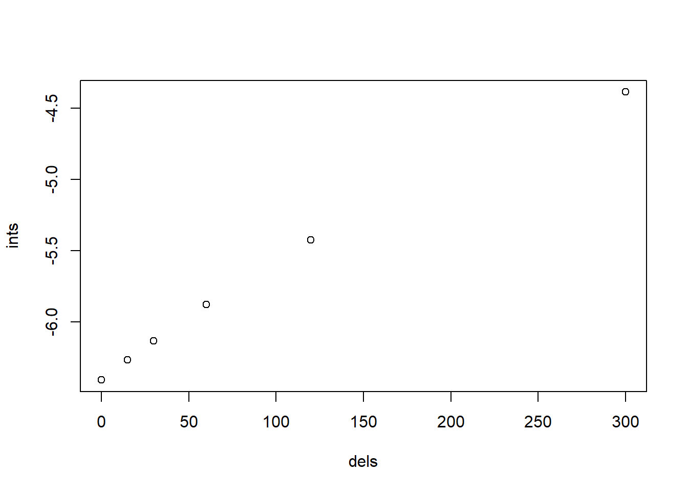

图 10.8: 基于 Cc 的不同延时下的截距

10.7.6 无光呼吸酶失活模块

该部分内容是在测量 ACi 曲线时检测 Rubisco 失活的影响 – 从激活状态的变化导致了多少的偏移？

10.7.6.1 数据构造

基于文献，假定 \(CO_2\) 从 400 ppm 降低至 5 ppm 时，激活率从 100% 降低至 80%。

#Assume that Rubisco activation state drops from 100% at 400 ppm to 80% at 5 ppm Cr (line 273 is Cr of 400, Cc of 297; 5ppm Cr is 25 ppm Cc) roughly from Salvucci et al 1986, arabidopsis; assume linear response

#不同的cr对应了不同的cc浓度，
#此为cc的变化范围（cr从400降低至5）
ccslope <- c(25, 297)
#酶的激活率变化
raslope <- c(0.80, 1.00)
#得到cc变化对应rubisco激活率变化的关系
ram1 <- lm(raslope ~ ccslope)
raslope <- coef(ram1)[2]
raint <- coef(ram1)[1]

#根据公式计算酶部分失活后各个参数
vora1 <- (raslope * Cc + raint) * Vomax * O2 / (O2 + Ko * (1 + Cc / Kc))
vcra1 <- (raslope * Cc + raint) * Vcmax * (Cc) / (Cc + Kco)
Ara1 <- vcra1 - 0.5 * vora1 - R
Aapparentra1 <- vcra1 - 0.5 * vora1
Cira1 <- Ara1 / gm + Cc
Cbra1 <- Ara1 / gsw + Cira1
Crra1 <- Ara1 / BLC + Cbra1

#失活后换算为分钟的变化斜率
Counter <- as.numeric(c(1:length(Cc)))
RateCr1model <- lm(Crra1 ~ Counter)
RateCr1 <- coef(RateCr1model)[2] * 60
RateCb1model <- lm(Cbra1 ~ Counter)
RateCb1 <- coef(RateCb1model)[2] * 60
RateCi1model <- lm(Cira1 ~ Counter)
RateCi1 <- coef(RateCi1model)[2] * 60
RateCcmodel <- lm(Cc ~ Counter)
RateCc <- coef(RateCcmodel)[2] * 60

#假定在5ppm时下降为40%
ccslope2 <- c(25, 297)
raslope2 <- c(0.40, 1.00)
ram2 <- lm(raslope2 ~ ccslope2)
raslope2 <- coef(ram2)[2]
raint2 <- coef(ram2)[1]

vora2 <-
  (raslope2 * Cc + raint2) * Vomax * O2 / (O2 + Ko * (1 + Cc / Kc)) 
vcra2 <- (raslope2 * Cc + raint2) * Vcmax * (Cc) / (Cc + Kco) 
Ara2 <- vcra2 - 0.5 * vora2 - R 
Aapparentra2 <- vcra2 - 0.5 * vora2 
Cira2 <- Ara2 / gm + Cc #umol mol-1
Cbra2 <- Ara2 / gsw + Cira2 #umol mol-1
Crra2 <- Ara2 / BLC + Cbra2 #umol mol-1
Counter <- as.numeric(c(1:length(Cc)))
RateCr2model <- lm(Crra2 ~ Counter)
RateCr2 <- coef(RateCr2model)[2] * 60 #umol mol-1 min-1
RateCb2model <- lm(Cbra2 ~ Counter)
RateCb2 <- coef(RateCb2model)[2] * 60 #umol mol-1 min-1
RateCi2model <- lm(Cira2 ~ Counter)
RateCi2 <- coef(RateCi2model)[2] * 60 #umol mol-1 min-1
RateCcmodel <- lm(Cc ~ Counter)
RateCc <- coef(RateCcmodel)[2] * 60 #umol mol-1 min-1

#假定在5ppm时下降为20%
ccslope3 <- c(25, 297)
raslope3 <- c(0.20, 1.00)
ram3 <- lm(raslope3 ~ ccslope3)
raslope3 <- coef(ram3)[2]
raint3 <- coef(ram3)[1]

vora3 <-
  (raslope3 * Cc + raint3) * Vomax * O2 / (O2 + Ko * (1 + Cc / Kc)) 
vcra3 <- (raslope3 * Cc + raint3) * Vcmax * (Cc) / (Cc + Kco) 
Ara3 <- vcra3 - 0.5 * vora3 - R 
Aapparentra3 <- vcra3 - 0.5 * vora3 
Cira3 <- Ara3 / gm + Cc 
Cbra3 <- Ara3 / gsw + Cira3 
Crra3 <- Ara3 / BLC + Cbra3 
Counter <- as.numeric(c(1:length(Cc)))
RateCr3model <- lm(Crra3 ~ Counter)
RateCr3 <- coef(RateCr3model)[2] * 60 
RateCb3model <- lm(Cbra3 ~ Counter)
RateCb3 <- coef(RateCb3model)[2] * 60 
RateCi3model <- lm(Cira3 ~ Counter)
RateCi3 <- coef(RateCi3model)[2] * 60 
RateCcmodel <- lm(Cc ~ Counter)
RateCc <- coef(RateCcmodel)[2] * 60 

Anet <- c(A, Ara1, Ara2, Ara3)
Aapp <- c(Aapparent, Aapparentra1, Aapparentra2, Aapparentra3)
Ccfull <- rep(Cc, 4)
Cifull <- c(Ci, Cira1, Cira2, Cira3)
Deactivation <-
  c(
    rep("None", length(A)),
    rep("Low", length(Ara1)),
    rep("Medium", length(Ara2)),
    rep("High", length(Ara3))
  )
RASdata <-
  as.data.frame(cbind(Anet, Aapp, Ccfull, Cifull, Deactivation))
write.csv(RASdata, "./data/RASdata.csv")

10.7.7 酶失活作图

data <- read.csv("./data/RASdata.csv")
data$Ccfull <- as.numeric(data$Ccfull)
data$Deactivation <- as.factor(data$Deactivation)

AnetCc <-
  ggplot(data, aes(x = Ccfull, y = Anet, colour = Deactivation)) +
  geom_point() +
  labs(x = expression(C[c] ~ "(" * mu * mol ~ mol ^ {
    -1
  } * ")"),
  y = expression(A[net] ~ "(" * mu * mol ~ m ^ {
    -2
  } ~ s ^ {
    -1
  } * ")")) +
  labs(colour = 'Deactivation') +
  scale_x_continuous(limits = c(25, 100),
                     breaks = c(25, 40, 55, 70, 85, 100)) +
  scale_y_continuous(limits = c(-5, 5)) +
  scale_colour_brewer(palette = 'Spectral') +
  geom_hline(yintercept = 0) +
  theme_bw() +
  theme(panel.grid.major = element_blank(),
        panel.grid.minor = element_blank())
AnetCc

## Warning: Removed 1205 rows containing missing values (geom_point).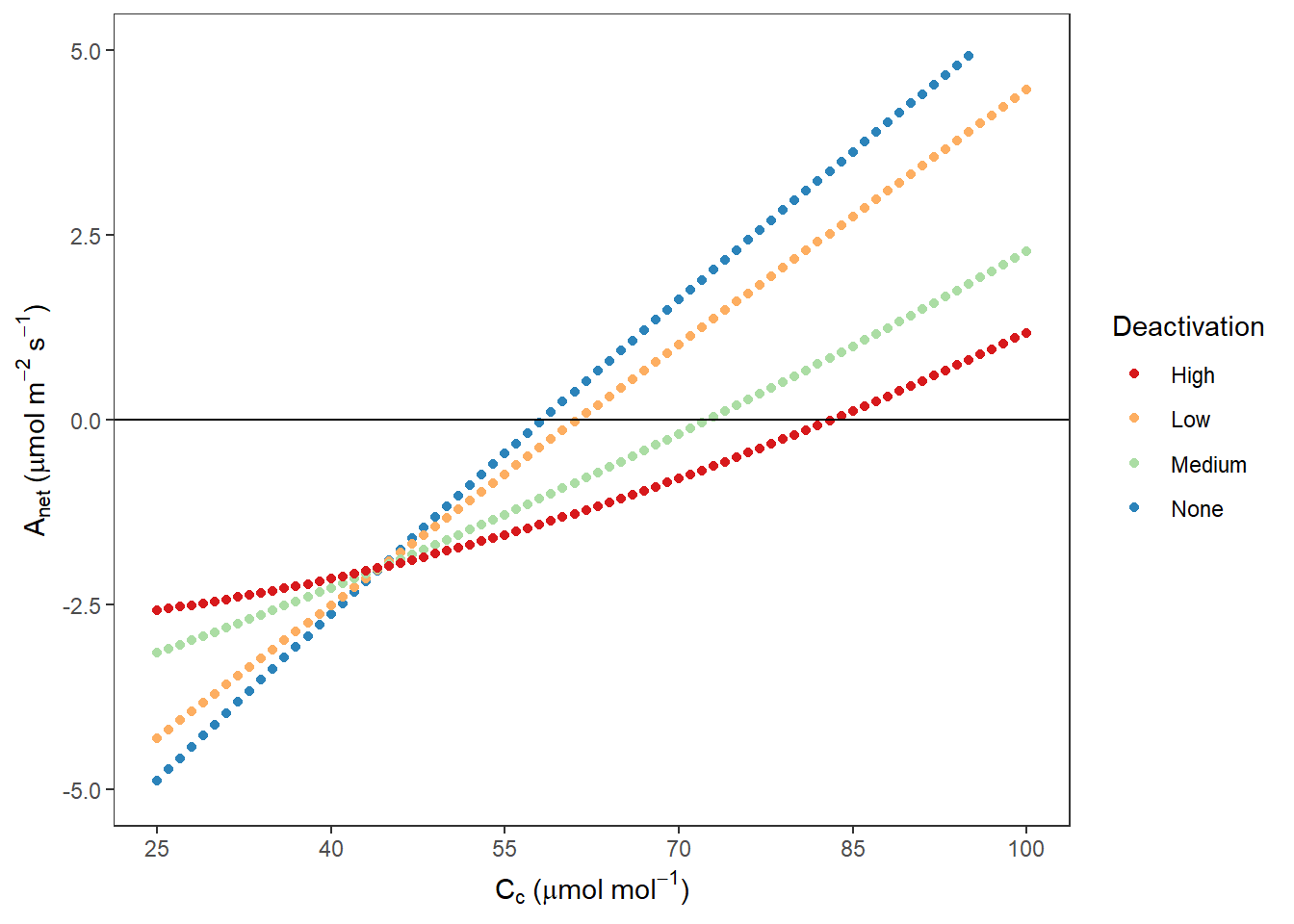

图 10.9: Rubisco 不同失活程度时 Anet VS Cc

AnetCi <-
  ggplot(data, aes(x = Cifull, y = Anet, colour = Deactivation)) +
  geom_point() +
  labs(x = expression(C[i] ~ "(" * mu * mol ~ mol ^ {
    -1
  } * ")"),
  y = expression(A[net] ~ "(" * mu * mol ~ m ^ {
    -2
  } ~ s ^ {
    -1
  } * ")")) +
  labs(colour = 'Deactivation') +
  scale_x_continuous(limits = c(25, 100),
                     breaks = c(25, 40, 55, 70, 85, 100)) +
  scale_y_continuous(limits = c(-5, 5)) +
  scale_colour_brewer(palette = 'Spectral') +
  geom_hline(yintercept = 0) +
  theme_bw() +
  theme(panel.grid.major = element_blank(),
        panel.grid.minor = element_blank())
AnetCi

## Warning: Removed 1230 rows containing missing values (geom_point).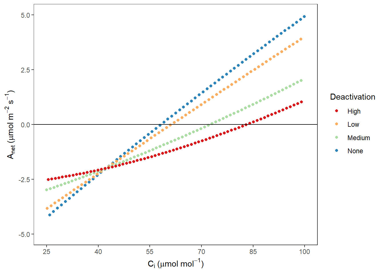

图 10.10: Rubisco 不同失活程度时 Anet VS Ci

AappCc <-
  ggplot(data, aes(x = Ccfull, y = Aapp, colour = Deactivation)) +
  geom_point() +
  labs(x = expression(C[c] ~ "(" * mu * mol ~ mol ^ {
    -1
  } * ")"),
  y = expression(A[apparent] ~ "(" * mu * mol ~ m ^ {
    -2
  } ~ s ^ {
    -1
  } * ")")) +
  labs(colour = 'Deactivation') +
  scale_x_continuous(limits = c(25, 75),
                     breaks = c(25, 35, 45, 55, 65, 75)) +
  scale_y_continuous(limits = c(-5, 5)) +
  scale_colour_brewer(palette = 'Spectral') +
  geom_hline(yintercept = 0) +
  theme_bw() +
  theme(panel.grid.major = element_blank(),
        panel.grid.minor = element_blank())
AappCc

## Warning: Removed 1300 rows containing missing values (geom_point).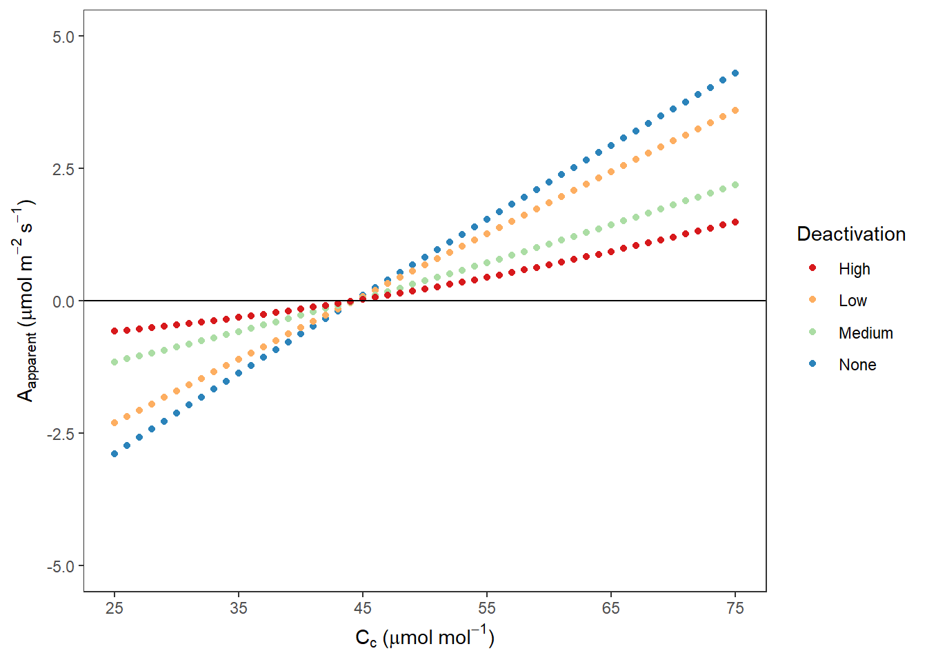

图 10.11: Rubisco 不同失活程度时 Aapp VS Cc

AappCi <-
  ggplot(data, aes(x = Cifull, y = Aapp, colour = Deactivation)) +
  geom_point() +
  labs(x = expression(C[i] ~ "(" * mu * mol ~ mol ^ {
    -1
  } * ")"),
  y = expression(A[apparent] ~ "(" * mu * mol ~ m ^ {
    -2
  } ~ s ^ {
    -1
  } * ")")) +
  labs(colour = 'Deactivation') +
  scale_x_continuous(limits = c(25, 75),
                     breaks = c(25, 35, 45, 55, 65, 75)) +
  scale_y_continuous(limits = c(-5, 5)) +
  scale_colour_brewer(palette = 'Spectral') +
  geom_hline(yintercept = 0) +
  theme_bw() +
  theme(panel.grid.major = element_blank(),
        panel.grid.minor = element_blank())
AappCi

## Warning: Removed 1321 rows containing missing values (geom_point).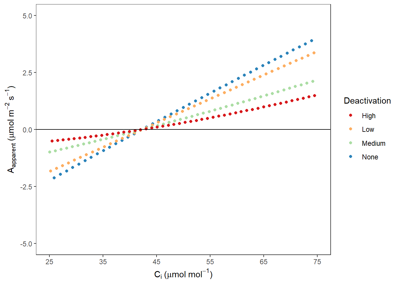

图 10.12: Rubisco 不同失活程度时 Aapp VS Ci

10.7.8 不同失活程度下补偿点计算

此部分内容同未失活状态相似，不在额外介绍，可参考 ?? 内容。

#Gamma
# For Ci-based estimates, only use Ci < 100
dataCi <- data[data$Cifull < 100, ]
dataCinone <- dataCi[dataCi$Deactivation == "None", ]
dataCilow <- dataCi[dataCi$Deactivation == "Low", ]
dataCimedium <- dataCi[dataCi$Deactivation == "Medium", ]
dataCihigh <- dataCi[dataCi$Deactivation == "High", ]
m1 <- lm(dataCinone$Anet ~ dataCinone$Cifull)
summary(m1)

## 
## Call:
## lm(formula = dataCinone$Anet ~ dataCinone$Cifull)
## 
## Residuals:
##      Min       1Q   Median       3Q      Max 
## -0.13165 -0.04518  0.01711  0.05408  0.06699 
## 
## Coefficients:
##                     Estimate Std. Error t value Pr(>|t|)    
## (Intercept)       -7.2248105  0.0199353  -362.4   <2e-16 ***
## dataCinone$Cifull  0.1228632  0.0003089   397.8   <2e-16 ***
## ---
## Signif. codes:  0 '***' 0.001 '**' 0.01 '*' 0.05 '.' 0.1 ' ' 1
## 
## Residual standard error: 0.06081 on 69 degrees of freedom
## Multiple R-squared:  0.9996, Adjusted R-squared:  0.9996 
## F-statistic: 1.582e+05 on 1 and 69 DF,  p-value: < 2.2e-16

Gammanone <- -m1$coefficients[1] / m1$coefficients[2]
m2 <- lm(dataCilow$Anet ~ dataCilow$Cifull)
summary(m2)

## 
## Call:
## lm(formula = dataCilow$Anet ~ dataCilow$Cifull)
## 
## Residuals:
##       Min        1Q    Median        3Q       Max 
## -0.034896 -0.011957  0.004499  0.014311  0.017726 
## 
## Coefficients:
##                    Estimate Std. Error t value Pr(>|t|)    
## (Intercept)      -6.444e+00  5.343e-03   -1206   <2e-16 ***
## dataCilow$Cifull  1.049e-01  8.341e-05    1258   <2e-16 ***
## ---
## Signif. codes:  0 '***' 0.001 '**' 0.01 '*' 0.05 '.' 0.1 ' ' 1
## 
## Residual standard error: 0.01609 on 69 degrees of freedom
## Multiple R-squared:      1,  Adjusted R-squared:      1 
## F-statistic: 1.582e+06 on 1 and 69 DF,  p-value: < 2.2e-16

Gammalow <- -m2$coefficients[1] / m2$coefficients[2]
m3 <- lm(dataCimedium$Anet ~ dataCimedium$Cifull)
summary(m3)

## 
## Call:
## lm(formula = dataCimedium$Anet ~ dataCimedium$Cifull)
## 
## Residuals:
##      Min       1Q   Median       3Q      Max 
## -0.09168 -0.07338 -0.02281  0.05893  0.18150 
## 
## Coefficients:
##                       Estimate Std. Error t value Pr(>|t|)    
## (Intercept)         -4.8015337  0.0277371  -173.1   <2e-16 ***
## dataCimedium$Cifull  0.0671064  0.0004311   155.7   <2e-16 ***
## ---
## Signif. codes:  0 '***' 0.001 '**' 0.01 '*' 0.05 '.' 0.1 ' ' 1
## 
## Residual standard error: 0.0832 on 71 degrees of freedom
## Multiple R-squared:  0.9971, Adjusted R-squared:  0.997 
## F-statistic: 2.423e+04 on 1 and 71 DF,  p-value: < 2.2e-16

Gammamedium <- -m3$coefficients[1] / m3$coefficients[2]
m4 <- lm(dataCihigh$Anet ~ dataCihigh$Cifull)
summary(m4)

## 
## Call:
## lm(formula = dataCihigh$Anet ~ dataCihigh$Cifull)
## 
## Residuals:
##      Min       1Q   Median       3Q      Max 
## -0.15430 -0.12508 -0.03863  0.10156  0.30621 
## 
## Coefficients:
##                     Estimate Std. Error t value Pr(>|t|)    
## (Intercept)       -3.9450658  0.0467537  -84.38   <2e-16 ***
## dataCihigh$Cifull  0.0473551  0.0007255   65.27   <2e-16 ***
## ---
## Signif. codes:  0 '***' 0.001 '**' 0.01 '*' 0.05 '.' 0.1 ' ' 1
## 
## Residual standard error: 0.1399 on 72 degrees of freedom
## Multiple R-squared:  0.9834, Adjusted R-squared:  0.9831 
## F-statistic:  4260 on 1 and 72 DF,  p-value: < 2.2e-16

Gammahigh <- -m4$coefficients[1] / m4$coefficients[2]

GammaCi <- c(Gammanone, Gammalow, Gammamedium, Gammahigh)

# For Cc-based estimates, only use Cc < 75
dataCc <- data[data$Ccfull < 75, ]
dataCcnone <- dataCc[dataCc$Deactivation == "None", ]
dataCclow <- dataCc[dataCc$Deactivation == "Low", ]
dataCcmedium <- dataCc[dataCc$Deactivation == "Medium", ]
dataCchigh <- dataCc[dataCc$Deactivation == "High", ]
m1 <- lm(dataCcnone$Anet ~ dataCcnone$Ccfull)
summary(m1)

## 
## Call:
## lm(formula = dataCcnone$Anet ~ dataCcnone$Ccfull)
## 
## Residuals:
##       Min        1Q    Median        3Q       Max 
## -0.075648 -0.025444  0.009857  0.031706  0.039431 
## 
## Coefficients:
##                     Estimate Std. Error t value Pr(>|t|)    
## (Intercept)       -8.4062011  0.0181852  -462.3   <2e-16 ***
## dataCcnone$Ccfull  0.1438710  0.0003527   407.9   <2e-16 ***
## ---
## Signif. codes:  0 '***' 0.001 '**' 0.01 '*' 0.05 '.' 0.1 ' ' 1
## 
## Residual standard error: 0.03599 on 48 degrees of freedom
## Multiple R-squared:  0.9997, Adjusted R-squared:  0.9997 
## F-statistic: 1.664e+05 on 1 and 48 DF,  p-value: < 2.2e-16

Gammanone <- -m1$coefficients[1] / m1$coefficients[2]
m2 <- lm(dataCclow$Anet ~ dataCclow$Ccfull)
summary(m2)

## 
## Call:
## lm(formula = dataCclow$Anet ~ dataCclow$Ccfull)
## 
## Residuals:
##       Min        1Q    Median        3Q       Max 
## -0.019617 -0.006598  0.002556  0.008222  0.010225 
## 
## Coefficients:
##                    Estimate Std. Error t value Pr(>|t|)    
## (Intercept)      -7.243e+00  4.716e-03   -1536   <2e-16 ***
## dataCclow$Ccfull  1.182e-01  9.146e-05    1292   <2e-16 ***
## ---
## Signif. codes:  0 '***' 0.001 '**' 0.01 '*' 0.05 '.' 0.1 ' ' 1
## 
## Residual standard error: 0.009333 on 48 degrees of freedom
## Multiple R-squared:      1,  Adjusted R-squared:      1 
## F-statistic: 1.67e+06 on 1 and 48 DF,  p-value: < 2.2e-16

Gammalow <- -m2$coefficients[1] / m2$coefficients[2]
m3 <- lm(dataCcmedium$Anet ~ dataCcmedium$Ccfull)
summary(m3)

## 
## Call:
## lm(formula = dataCcmedium$Anet ~ dataCcmedium$Ccfull)
## 
## Residuals:
##      Min       1Q   Median       3Q      Max 
## -0.04819 -0.03875 -0.01205  0.03109  0.09244 
## 
## Coefficients:
##                      Estimate Std. Error t value Pr(>|t|)    
## (Intercept)         -4.917283   0.022223  -221.3   <2e-16 ***
## dataCcmedium$Ccfull  0.066832   0.000431   155.1   <2e-16 ***
## ---
## Signif. codes:  0 '***' 0.001 '**' 0.01 '*' 0.05 '.' 0.1 ' ' 1
## 
## Residual standard error: 0.04398 on 48 degrees of freedom
## Multiple R-squared:  0.998,  Adjusted R-squared:  0.998 
## F-statistic: 2.404e+04 on 1 and 48 DF,  p-value: < 2.2e-16

Gammamedium <- -m3$coefficients[1] / m3$coefficients[2]
m4 <- lm(dataCchigh$Anet ~ dataCchigh$Ccfull)
summary(m4)

## 
## Call:
## lm(formula = dataCchigh$Anet ~ dataCchigh$Ccfull)
## 
## Residuals:
##      Min       1Q   Median       3Q      Max 
## -0.07739 -0.06223 -0.01935  0.04994  0.14847 
## 
## Coefficients:
##                     Estimate Std. Error t value Pr(>|t|)    
## (Intercept)       -3.7543099  0.0356922 -105.19   <2e-16 ***
## dataCchigh$Ccfull  0.0411528  0.0006922   59.45   <2e-16 ***
## ---
## Signif. codes:  0 '***' 0.001 '**' 0.01 '*' 0.05 '.' 0.1 ' ' 1
## 
## Residual standard error: 0.07064 on 48 degrees of freedom
## Multiple R-squared:  0.9866, Adjusted R-squared:  0.9863 
## F-statistic:  3534 on 1 and 48 DF,  p-value: < 2.2e-16

Gammahigh <- -m4$coefficients[1] / m4$coefficients[2]

GammaCc <- c(Gammanone, Gammalow, Gammamedium, Gammahigh)

#GammaStar
# For Ci-based estimates, only use Ci < 100
dataCi <- data[data$Cifull < 100, ]
dataCinone <- dataCi[dataCi$Deactivation == "None", ]
dataCilow <- dataCi[dataCi$Deactivation == "Low", ]
dataCimedium <- dataCi[dataCi$Deactivation == "Medium", ]
dataCihigh <- dataCi[dataCi$Deactivation == "High", ]
m1 <- lm(dataCinone$Aapp ~ dataCinone$Cifull)
summary(m1)

## 
## Call:
## lm(formula = dataCinone$Aapp ~ dataCinone$Cifull)
## 
## Residuals:
##      Min       1Q   Median       3Q      Max 
## -0.13165 -0.04518  0.01711  0.05408  0.06699 
## 
## Coefficients:
##                     Estimate Std. Error t value Pr(>|t|)    
## (Intercept)       -5.2248105  0.0199353  -262.1   <2e-16 ***
## dataCinone$Cifull  0.1228632  0.0003089   397.8   <2e-16 ***
## ---
## Signif. codes:  0 '***' 0.001 '**' 0.01 '*' 0.05 '.' 0.1 ' ' 1
## 
## Residual standard error: 0.06081 on 69 degrees of freedom
## Multiple R-squared:  0.9996, Adjusted R-squared:  0.9996 
## F-statistic: 1.582e+05 on 1 and 69 DF,  p-value: < 2.2e-16

Gammastarnone <- -m1$coefficients[1] / m1$coefficients[2]
m2 <- lm(dataCilow$Aapp ~ dataCilow$Cifull)
summary(m2)

## 
## Call:
## lm(formula = dataCilow$Aapp ~ dataCilow$Cifull)
## 
## Residuals:
##       Min        1Q    Median        3Q       Max 
## -0.034896 -0.011957  0.004499  0.014311  0.017726 
## 
## Coefficients:
##                    Estimate Std. Error t value Pr(>|t|)    
## (Intercept)      -4.444e+00  5.343e-03  -831.7   <2e-16 ***
## dataCilow$Cifull  1.049e-01  8.341e-05  1257.8   <2e-16 ***
## ---
## Signif. codes:  0 '***' 0.001 '**' 0.01 '*' 0.05 '.' 0.1 ' ' 1
## 
## Residual standard error: 0.01609 on 69 degrees of freedom
## Multiple R-squared:      1,  Adjusted R-squared:      1 
## F-statistic: 1.582e+06 on 1 and 69 DF,  p-value: < 2.2e-16

Gammastarlow <- -m2$coefficients[1] / m2$coefficients[2]
m3 <- lm(dataCimedium$Aapp ~ dataCimedium$Cifull)
summary(m3)

## 
## Call:
## lm(formula = dataCimedium$Aapp ~ dataCimedium$Cifull)
## 
## Residuals:
##      Min       1Q   Median       3Q      Max 
## -0.09168 -0.07338 -0.02281  0.05893  0.18150 
## 
## Coefficients:
##                       Estimate Std. Error t value Pr(>|t|)    
## (Intercept)         -2.8015337  0.0277371  -101.0   <2e-16 ***
## dataCimedium$Cifull  0.0671064  0.0004311   155.7   <2e-16 ***
## ---
## Signif. codes:  0 '***' 0.001 '**' 0.01 '*' 0.05 '.' 0.1 ' ' 1
## 
## Residual standard error: 0.0832 on 71 degrees of freedom
## Multiple R-squared:  0.9971, Adjusted R-squared:  0.997 
## F-statistic: 2.423e+04 on 1 and 71 DF,  p-value: < 2.2e-16

Gammastarmedium <- -m3$coefficients[1] / m3$coefficients[2]
m4 <- lm(dataCihigh$Aapp ~ dataCihigh$Cifull)
summary(m4)

## 
## Call:
## lm(formula = dataCihigh$Aapp ~ dataCihigh$Cifull)
## 
## Residuals:
##      Min       1Q   Median       3Q      Max 
## -0.15430 -0.12508 -0.03863  0.10156  0.30621 
## 
## Coefficients:
##                     Estimate Std. Error t value Pr(>|t|)    
## (Intercept)       -1.9450658  0.0467537  -41.60   <2e-16 ***
## dataCihigh$Cifull  0.0473551  0.0007255   65.27   <2e-16 ***
## ---
## Signif. codes:  0 '***' 0.001 '**' 0.01 '*' 0.05 '.' 0.1 ' ' 1
## 
## Residual standard error: 0.1399 on 72 degrees of freedom
## Multiple R-squared:  0.9834, Adjusted R-squared:  0.9831 
## F-statistic:  4260 on 1 and 72 DF,  p-value: < 2.2e-16

Gammastarhigh <- -m4$coefficients[1] / m4$coefficients[2]

GammastarCi <-
  c(Gammastarnone, Gammastarlow, Gammastarmedium, Gammastarhigh)

# For Cc-based estimates, only use Cc < 75
dataCc <- data[data$Ccfull < 75, ]
dataCcnone <- dataCc[dataCc$Deactivation == "None", ]
dataCclow <- dataCc[dataCc$Deactivation == "Low", ]
dataCcmedium <- dataCc[dataCc$Deactivation == "Medium", ]
dataCchigh <- dataCc[dataCc$Deactivation == "High", ]
m1 <- lm(dataCcnone$Aapp ~ dataCcnone$Ccfull)
summary(m1)

## 
## Call:
## lm(formula = dataCcnone$Aapp ~ dataCcnone$Ccfull)
## 
## Residuals:
##       Min        1Q    Median        3Q       Max 
## -0.075648 -0.025444  0.009857  0.031706  0.039431 
## 
## Coefficients:
##                     Estimate Std. Error t value Pr(>|t|)    
## (Intercept)       -6.4062011  0.0181852  -352.3   <2e-16 ***
## dataCcnone$Ccfull  0.1438710  0.0003527   407.9   <2e-16 ***
## ---
## Signif. codes:  0 '***' 0.001 '**' 0.01 '*' 0.05 '.' 0.1 ' ' 1
## 
## Residual standard error: 0.03599 on 48 degrees of freedom
## Multiple R-squared:  0.9997, Adjusted R-squared:  0.9997 
## F-statistic: 1.664e+05 on 1 and 48 DF,  p-value: < 2.2e-16

Gammastarnone <- -m1$coefficients[1] / m1$coefficients[2]
m2 <- lm(dataCclow$Aapp ~ dataCclow$Ccfull)
summary(m2)

## 
## Call:
## lm(formula = dataCclow$Aapp ~ dataCclow$Ccfull)
## 
## Residuals:
##       Min        1Q    Median        3Q       Max 
## -0.019617 -0.006598  0.002556  0.008222  0.010225 
## 
## Coefficients:
##                    Estimate Std. Error t value Pr(>|t|)    
## (Intercept)      -5.243e+00  4.716e-03   -1112   <2e-16 ***
## dataCclow$Ccfull  1.182e-01  9.146e-05    1292   <2e-16 ***
## ---
## Signif. codes:  0 '***' 0.001 '**' 0.01 '*' 0.05 '.' 0.1 ' ' 1
## 
## Residual standard error: 0.009333 on 48 degrees of freedom
## Multiple R-squared:      1,  Adjusted R-squared:      1 
## F-statistic: 1.67e+06 on 1 and 48 DF,  p-value: < 2.2e-16

Gammastarlow <- -m2$coefficients[1] / m2$coefficients[2]
m3 <- lm(dataCcmedium$Aapp ~ dataCcmedium$Ccfull)
summary(m3)

## 
## Call:
## lm(formula = dataCcmedium$Aapp ~ dataCcmedium$Ccfull)
## 
## Residuals:
##      Min       1Q   Median       3Q      Max 
## -0.04819 -0.03875 -0.01205  0.03109  0.09244 
## 
## Coefficients:
##                      Estimate Std. Error t value Pr(>|t|)    
## (Intercept)         -2.917283   0.022223  -131.3   <2e-16 ***
## dataCcmedium$Ccfull  0.066832   0.000431   155.1   <2e-16 ***
## ---
## Signif. codes:  0 '***' 0.001 '**' 0.01 '*' 0.05 '.' 0.1 ' ' 1
## 
## Residual standard error: 0.04398 on 48 degrees of freedom
## Multiple R-squared:  0.998,  Adjusted R-squared:  0.998 
## F-statistic: 2.404e+04 on 1 and 48 DF,  p-value: < 2.2e-16

Gammastarmedium <- -m3$coefficients[1] / m3$coefficients[2]
m4 <- lm(dataCchigh$Aapp ~ dataCchigh$Ccfull)
summary(m4)

## 
## Call:
## lm(formula = dataCchigh$Aapp ~ dataCchigh$Ccfull)
## 
## Residuals:
##      Min       1Q   Median       3Q      Max 
## -0.07739 -0.06223 -0.01935  0.04994  0.14847 
## 
## Coefficients:
##                     Estimate Std. Error t value Pr(>|t|)    
## (Intercept)       -1.7543099  0.0356922  -49.15   <2e-16 ***
## dataCchigh$Ccfull  0.0411528  0.0006922   59.45   <2e-16 ***
## ---
## Signif. codes:  0 '***' 0.001 '**' 0.01 '*' 0.05 '.' 0.1 ' ' 1
## 
## Residual standard error: 0.07064 on 48 degrees of freedom
## Multiple R-squared:  0.9866, Adjusted R-squared:  0.9863 
## F-statistic:  3534 on 1 and 48 DF,  p-value: < 2.2e-16

Gammastarhigh <- -m4$coefficients[1] / m4$coefficients[2]

GammastarCc <-
  c(Gammastarnone, Gammastarlow, Gammastarmedium, Gammastarhigh)

Deactivation2 <- c("None", "Low", "Medium", "High")
RAScomps <-
  as.data.frame(cbind(Deactivation2, GammaCc, GammaCi, GammastarCc, GammastarCi))
write.csv(RAScomps, "./data/RAScomps.csv")

10.8 时间延迟的扩散限制

对于扩散限制，下面的内容比较了多速率 RACiR 和标准 ACi 曲线的差别，比较实在有光呼吸和没有光呼吸的两种情况。对于没有扩散限制的表观光合速，采用了已知质量的碱石灰药品，放置于 1.7 ml 的微量离心管内，然后将其置于荧光叶室内部模拟叶片，此时叶室环境控制与其他实验不同，此时不再控制 H2OR。RACiR 测试从 500 到 0 的变化，不同样品的测量是随机的。

下面内容采用了一定的假设，来计算扩散的时间。

#Equations from Campbell & Norman, 1998
#We are taking a simple approach to calculating diffusion times.
#Here we make the simplifying assumption that diffusion is pure, planar
#Diffusion, such that:
#gtot = phat * D / deltaZ
#where gtot is total conductance, phat is molar density of air in mol /m^3,
#D is diffusion coefficient in m2/s, deltaZ is pathlength in m
#Since PV = NRT, N/V = P/RT
#T in K, R in J K-1 mol-1, P in Pa

#phat = Patm/(RT)
phat = 100000 / (8.314 * 298.15)

#We also assume a linear pathlength
#Note, if diffusion is nonlinear or nonplanar, it will affect the value determined
#for D from this equation.

#D = gtot * deltaZ / phat

#Diffusion time, t, varies with D and deltaZ such that:

#t = (deltaZ)^2 / D

#So

#t = (deltaZ)^2 / (gtot * deltaZ / phat)

#If we assume mean diffusion pathlength of 1/2 lamina thickness,
#then Onoda et al. 2011 lamina thicknesses of: median 0.22 mm (0.11 to 0.74 for 95% CI)
#becomes 0.11 mm (0.055 to 0.37) for estimated deltaZ

#Convert pathlength to m
dZlow <- 0.055 / 1000
dZmedian <- 0.11 / 1000
dZhigh <- 0.37 / 1000

下面的内容是对边界层导度和气孔导度等赋值，由此而计算出其他所需要的参数：

#Mesophyll Conductance
BLC <- 2 #mol m-2 s-1
gsw <- 0.4 #mol m-2 s-1

# 无限制的叶肉导度，并以此计算ci等
gm1 <- 1 #mol m-2 s-1
Ci1 <- A / gm1 + Cc #umol mol-1
Cim1 <- Ci1
Cb1 <- A / gsw + Ci1 #umol mol-1
Cr1 <- A / BLC + Cb1 #umol mol-1
#根据斜率计算达到 100 ppm min-1 时记录数据的个数
Counter <- as.numeric(c(1:length(Cc)))
RateCrmodel <- lm(Cr1 ~ Counter)
x1 <- 100 / coef(RateCrmodel)[2] 
RateCr1 <- coef(RateCrmodel)[2] * x1 #umol mol-1 min-1
#计算ci，Cc等达到100ppm min-1 时数据的个数
RateCbmodel <- lm(Cb1 ~ Counter)
RateCb1 <- coef(RateCbmodel)[2] * x1 #umol mol-1 min-1
RateCimodel <- lm(Ci1 ~ Counter)
RateCi1 <- coef(RateCimodel)[2] * x1 #umol mol-1 min-1
RateCcmodel <- lm(Cc ~ Counter)
RateCc1 <- coef(RateCcmodel)[2] * x1 #umol mol-1 min-1
#总的阻力
res1 <- 1 / gm1 + 1 / BLC + 1 / gsw

#不同的叶肉导度计算其他参数
gm2 <- 2 #mol m-2 s-1
Ci2 <- A / gm2 + Cc #umol mol-1
Cim2 <- Ci2
Cb2 <- A / gsw + Ci2 #umol mol-1
Cr2 <- A / BLC + Cb2 #umol mol-1
Counter <- as.numeric(c(1:length(Cc)))
RateCrmodel <- lm(Cr2 ~ Counter)
x2 <- 100 / coef(RateCrmodel)[2] 
RateCr2 <- coef(RateCrmodel)[2] * x2 #umol mol-1 min-1
RateCbmodel <- lm(Cb2 ~ Counter)
RateCb2 <- coef(RateCbmodel)[2] * x2 #umol mol-1 min-1
RateCimodel <- lm(Ci2 ~ Counter)
RateCi2 <- coef(RateCimodel)[2] * x2 #umol mol-1 min-1
RateCcmodel <- lm(Cc ~ Counter)
RateCc2 <- coef(RateCcmodel)[2] * x2 #umol mol-1 min-1
res2 <- 1 / gm2 + 1 / BLC + 1 / gsw

#再次计算不同导度下的数值
gm4 <- 4 #mol m-2 s-1
Ci4 <- A / gm4 + Cc #umol mol-1
Cim4 <- Ci4
Cb4 <- A / gsw + Ci4 #umol mol-1
Cr4 <- A / BLC + Cb4 #umol mol-1
Counter <- as.numeric(c(1:length(Cc)))
RateCrmodel <- lm(Cr4 ~ Counter)
x4 <- 100 / coef(RateCrmodel)[2]
RateCr4 <- coef(RateCrmodel)[2] * x4 #umol mol-1 min-1
RateCbmodel <- lm(Cb4 ~ Counter)
RateCb4 <- coef(RateCbmodel)[2] * x4 #umol mol-1 min-1
RateCimodel <- lm(Ci4 ~ Counter)
RateCi4 <- coef(RateCimodel)[2] * x4 #umol mol-1 min-1
RateCcmodel <- lm(Cc ~ Counter)
RateCc4 <- coef(RateCcmodel)[2] * x4 #umol mol-1 min-1
res4 <- 1 / gm4 + 1 / BLC + 1 / gsw

#再次计算不同导度下的数值
gm05 <- 0.5 #mol m-2 s-1
Ci05 <- A / gm05 + Cc #umol mol-1
Cim05 <- Ci05
Cb05 <- A / gsw + Ci05 #umol mol-1
Cr05 <- A / BLC + Cb05 #umol mol-1
Counter <- as.numeric(c(1:length(Cc)))
RateCrmodel <- lm(Cr05 ~ Counter)
x05 <- 100 / coef(RateCrmodel)[2]
RateCr05 <- coef(RateCrmodel)[2] * x05 #umol mol-1 min-1
RateCbmodel <- lm(Cb05 ~ Counter)
RateCb05 <- coef(RateCbmodel)[2] * x05 #umol mol-1 min-1
RateCimodel <- lm(Ci05 ~ Counter)
RateCi05 <- coef(RateCimodel)[2] * x05 #umol mol-1 min-1
RateCcmodel <- lm(Cc ~ Counter)
RateCc05 <- coef(RateCcmodel)[2] * x05 #umol mol-1 min-1
res05 <- 1 / gm05 + 1 / BLC + 1 / gsw

#正常的叶肉导度数据计算其他参数
gm025 <- 0.25 #mol m-2 s-1
Ci025 <- A / gm025 + Cc #umol mol-1
Cim025 <- Ci025
Cb025 <- A / gsw + Ci025 #umol mol-1
Cr025 <- A / BLC + Cb025 #umol mol-1
Counter <- as.numeric(c(1:length(Cc)))
RateCrmodel <- lm(Cr025 ~ Counter)
x025 <- 100 / coef(RateCrmodel)[2]
RateCr025 <- coef(RateCrmodel)[2] * x025 #umol mol-1 min-1
RateCbmodel <- lm(Cb025 ~ Counter)
RateCb025 <- coef(RateCbmodel)[2] * x025 #umol mol-1 min-1
RateCimodel <- lm(Ci025 ~ Counter)
RateCi025 <- coef(RateCimodel)[2] * x025 #umol mol-1 min-1
RateCcmodel <- lm(Cc ~ Counter)
RateCc025 <- coef(RateCcmodel)[2] * x025 #umol mol-1 min-1
res025 <- 1 / gm025 + 1 / BLC + 1 / gsw

#另一个正常的叶肉导度
gm0125 <- 0.125 #mol m-2 s-1
Ci0125 <- A / gm0125 + Cc #umol mol-1
Cim0125 <- Ci0125
Cb0125 <- A / gsw + Ci0125 #umol mol-1
Cr0125 <- A / BLC + Cb0125 #umol mol-1
Counter <- as.numeric(c(1:length(Cc)))
RateCrmodel <- lm(Cr0125 ~ Counter)
x0125 <- 100 / coef(RateCrmodel)[2]
RateCr0125 <- coef(RateCrmodel)[2] * x0125 #umol mol-1 min-1
RateCbmodel <- lm(Cb0125 ~ Counter)
RateCb0125 <- coef(RateCbmodel)[2] * x0125 #umol mol-1 min-1
RateCimodel <- lm(Ci0125 ~ Counter)
RateCi0125 <- coef(RateCimodel)[2] * x0125 #umol mol-1 min-1
RateCcmodel <- lm(Cc ~ Counter)
RateCc0125 <- coef(RateCcmodel)[2] * x0125 #umol mol-1 min-1
res0125 <- 1 / gm0125 + 1 / BLC + 1 / gsw

#利用不同叶肉导度的数据计算结果构造数据
Ratesgm <-
  c(RateCc0125, RateCc025, RateCc05, RateCc1, RateCc2, RateCc4)
gmval <- c(0.125, 0.25, 0.5, 1, 2, 4)
totalresgm <- c(res0125, res025, res05, res1, res2, res4)
resistance <-
  c(
    rep(res0125, 376),
    rep(res025, 376),
    rep(res05, 376),
    rep(res1, 376),
    rep(res2, 376),
    rep(res4, 376)
  )

#其余部分与上面类似
#此时采用不同的气孔导度构建数据
BLC <- 2 #mol m-2 s-1
gm <- 1 #mol m-2 s-1

gsw <- 0.4 #mol m-2 s-1
Ci1 <- A / gm + Cc #umol mol-1
Cis04 <- Ci1
Cb1 <- A / gsw + Ci1 #umol mol-1
Cr1 <- A / BLC + Cb1 #umol mol-1
Counter <- as.numeric(c(1:length(Cc)))
RateCrmodel <- lm(Cr1 ~ Counter)
x1 <- 100 / coef(RateCrmodel)[2] 
RateCr1 <- coef(RateCrmodel)[2] * x1 #umol mol-1 min-1
RateCbmodel <- lm(Cb1 ~ Counter)
RateCb1 <- coef(RateCbmodel)[2] * x1 #umol mol-1 min-1
RateCimodel <- lm(Ci1 ~ Counter)
RateCi1 <- coef(RateCimodel)[2] * x1 #umol mol-1 min-1
RateCcmodel <- lm(Cc ~ Counter)
RateCc04 <- coef(RateCcmodel)[2] * x1 #umol mol-1 min-1
res04 <- 1 / gm + 1 / BLC + 1 / gsw

gsw <- 0.2 #mol m-2 s-1
Ci1 <- A / gm + Cc #umol mol-1
Cis02 <- Ci1
Cb1 <- A / gsw + Ci1 #umol mol-1
Cr1 <- A / BLC + Cb1 #umol mol-1
Counter <- as.numeric(c(1:length(Cc)))
RateCrmodel <- lm(Cr1 ~ Counter)
x1 <- 100 / coef(RateCrmodel)[2]
RateCr1 <- coef(RateCrmodel)[2] * x1 #umol mol-1 min-1
RateCbmodel <- lm(Cb1 ~ Counter)
RateCb1 <- coef(RateCbmodel)[2] * x1 #umol mol-1 min-1
RateCimodel <- lm(Ci1 ~ Counter)
RateCi1 <- coef(RateCimodel)[2] * x1 #umol mol-1 min-1
RateCcmodel <- lm(Cc ~ Counter)
RateCc02 <- coef(RateCcmodel)[2] * x1 #umol mol-1 min-1
res02 <- 1 / gm + 1 / BLC + 1 / gsw

gsw <- 0.1 #mol m-2 s-1
Ci1 <- A / gm + Cc #umol mol-1
Cis01 <- Ci1
Cb1 <- A / gsw + Ci1 #umol mol-1
Cr1 <- A / BLC + Cb1 #umol mol-1
Counter <- as.numeric(c(1:length(Cc)))
RateCrmodel <- lm(Cr1 ~ Counter)
x1 <- 100 / coef(RateCrmodel)[2]
RateCr1 <- coef(RateCrmodel)[2] * x1 #umol mol-1 min-1
RateCbmodel <- lm(Cb1 ~ Counter)
RateCb1 <- coef(RateCbmodel)[2] * x1 #umol mol-1 min-1
RateCimodel <- lm(Ci1 ~ Counter)
RateCi1 <- coef(RateCimodel)[2] * x1 #umol mol-1 min-1
RateCcmodel <- lm(Cc ~ Counter)
RateCc01 <- coef(RateCcmodel)[2] * x1 #umol mol-1 min-1
res01 <- 1 / gm + 1 / BLC + 1 / gsw

gsw <- 0.05 #mol m-2 s-1
Ci1 <- A / gm + Cc #umol mol-1
Cis05 <- Ci1
Cb1 <- A / gsw + Ci1 #umol mol-1
Cr1 <- A / BLC + Cb1 #umol mol-1
Counter <- as.numeric(c(1:length(Cc)))
RateCrmodel <- lm(Cr1 ~ Counter)
x1 <- 100 / coef(RateCrmodel)[2]
RateCr1 <- coef(RateCrmodel)[2] * x1 #umol mol-1 min-1
RateCbmodel <- lm(Cb1 ~ Counter)
RateCb1 <- coef(RateCbmodel)[2] * x1 #umol mol-1 min-1
RateCimodel <- lm(Ci1 ~ Counter)
RateCi1 <- coef(RateCimodel)[2] * x1 #umol mol-1 min-1
RateCcmodel <- lm(Cc ~ Counter)
RateCc005 <- coef(RateCcmodel)[2] * x1 #umol mol-1 min-1
res005 <- 1 / gm + 1 / BLC + 1 / gsw

gsw <- 0.025 #mol m-2 s-1
Ci1 <- A / gm + Cc #umol mol-1
Cis0025 <- Ci1
Cb1 <- A / gsw + Ci1 #umol mol-1
Cr1 <- A / BLC + Cb1 #umol mol-1
Counter <- as.numeric(c(1:length(Cc)))
RateCrmodel <- lm(Cr1 ~ Counter)
x1 <- 100 / coef(RateCrmodel)[2]
RateCr1 <- coef(RateCrmodel)[2] * x1 #umol mol-1 min-1
RateCbmodel <- lm(Cb1 ~ Counter)
RateCb1 <- coef(RateCbmodel)[2] * x1 #umol mol-1 min-1
RateCimodel <- lm(Ci1 ~ Counter)
RateCi1 <- coef(RateCimodel)[2] * x1 #umol mol-1 min-1
RateCcmodel <- lm(Cc ~ Counter)
RateCc0025 <- coef(RateCcmodel)[2] * x1 #umol mol-1 min-1
res0025 <- 1 / gm + 1 / BLC + 1 / gsw

Ratesgsw <- c(RateCc0025, RateCc005, RateCc01, RateCc02, RateCc04)
gswvals <- c(0.025, 0.05, 0.1, 0.2, 0.4)
totalresgsw <- c(res0025, res005, res01, res02, res04)

# 下面的代码是采用不同的边界层导度
# 含义与上面代码相似
gm <- 1 #mol m-2 s-1
gsw <- 0.4 #mol m-2 s-1

BLC <- 2 #mol m-2 s-1

Ci1 <- A / gm + Cc #umol mol-1
Cib2 <- Ci1
Cb1 <- A / gsw + Ci1 #umol mol-1
Cr1 <- A / BLC + Cb1 #umol mol-1
Counter <- as.numeric(c(1:length(Cc)))
RateCrmodel <- lm(Cr1 ~ Counter)
x1 <- 100 / coef(RateCrmodel)[2]
RateCr1 <- coef(RateCrmodel)[2] * x1 #umol mol-1 min-1
RateCbmodel <- lm(Cb1 ~ Counter)
RateCb1 <- coef(RateCbmodel)[2] * x1 #umol mol-1 min-1
RateCimodel <- lm(Ci1 ~ Counter)
RateCi1 <- coef(RateCimodel)[2] * x1 #umol mol-1 min-1
RateCcmodel <- lm(Cc ~ Counter)
RateCc2 <- coef(RateCcmodel)[2] * x1 #umol mol-1 min-1
res2 <- 1 / gm + 1 / BLC + 1 / gsw

BLC <- 4 #mol m-2 s-1

Ci1 <- A / gm + Cc #umol mol-1
Cib4 <- Ci1
Cb1 <- A / gsw + Ci1 #umol mol-1
Cr1 <- A / BLC + Cb1 #umol mol-1
Counter <- as.numeric(c(1:length(Cc)))
RateCrmodel <- lm(Cr1 ~ Counter)
x1 <- 100 / coef(RateCrmodel)[2]
RateCr1 <- coef(RateCrmodel)[2] * x1 #umol mol-1 min-1
RateCbmodel <- lm(Cb1 ~ Counter)
RateCb1 <- coef(RateCbmodel)[2] * x1 #umol mol-1 min-1
RateCimodel <- lm(Ci1 ~ Counter)
RateCi1 <- coef(RateCimodel)[2] * x1 #umol mol-1 min-1
RateCcmodel <- lm(Cc ~ Counter)
RateCc4 <- coef(RateCcmodel)[2] * x1 #umol mol-1 min-1
res4 <- 1 / gm + 1 / BLC + 1 / gsw

BLC <- 1 #mol m-2 s-1

Ci1 <- A / gm + Cc #umol mol-1
Cib1 <- Ci1
Cb1 <- A / gsw + Ci1 #umol mol-1
Cr1 <- A / BLC + Cb1 #umol mol-1
Counter <- as.numeric(c(1:length(Cc)))
RateCrmodel <- lm(Cr1 ~ Counter)
x1 <- 100 / coef(RateCrmodel)[2]
RateCr1 <- coef(RateCrmodel)[2] * x1 #umol mol-1 min-1
RateCbmodel <- lm(Cb1 ~ Counter)
RateCb1 <- coef(RateCbmodel)[2] * x1 #umol mol-1 min-1
RateCimodel <- lm(Ci1 ~ Counter)
RateCi1 <- coef(RateCimodel)[2] * x1 #umol mol-1 min-1
RateCcmodel <- lm(Cc ~ Counter)
RateCc1 <- coef(RateCcmodel)[2] * x1 #umol mol-1 min-1
res1 <- 1 / gm + 1 / BLC + 1 / gsw

BLC <- 0.5 #mol m-2 s-1

Ci1 <- A / gm + Cc #umol mol-1
Cb1 <- A / gsw + Ci1 #umol mol-1
Cib05 <- Ci1
Cr1 <- A / BLC + Cb1 #umol mol-1
Counter <- as.numeric(c(1:length(Cc)))
RateCrmodel <- lm(Cr1 ~ Counter)
x1 <- 100 / coef(RateCrmodel)[2]
RateCr1 <- coef(RateCrmodel)[2] * x1 #umol mol-1 min-1
RateCbmodel <- lm(Cb1 ~ Counter)
RateCb1 <- coef(RateCbmodel)[2] * x1 #umol mol-1 min-1
RateCimodel <- lm(Ci1 ~ Counter)
RateCi1 <- coef(RateCimodel)[2] * x1 #umol mol-1 min-1
RateCcmodel <- lm(Cc ~ Counter)
RateCc05 <- coef(RateCcmodel)[2] * x1 #umol mol-1 min-1
res05 <- 1 / gm + 1 / BLC + 1 / gsw

BLC <- 0.25 #mol m-2 s-1

Ci1 <- A / gm + Cc #umol mol-1
Cb1 <- A / gsw + Ci1 #umol mol-1
Cib025 <- Ci1
Cr1 <- A / BLC + Cb1 #umol mol-1
Counter <- as.numeric(c(1:length(Cc)))
RateCrmodel <- lm(Cr1 ~ Counter)
x1 <- 100 / coef(RateCrmodel)[2]
RateCr1 <- coef(RateCrmodel)[2] * x1 #umol mol-1 min-1
RateCbmodel <- lm(Cb1 ~ Counter)
RateCb1 <- coef(RateCbmodel)[2] * x1 #umol mol-1 min-1
RateCimodel <- lm(Ci1 ~ Counter)
RateCi1 <- coef(RateCimodel)[2] * x1 #umol mol-1 min-1
RateCcmodel <- lm(Cc ~ Counter)
RateCc025 <- coef(RateCcmodel)[2] * x1 #umol mol-1 min-1
res025 <- 1 / gm + 1 / BLC + 1 / gsw

BLCRates <- c(RateCc025, RateCc05, RateCc1, RateCc2, RateCc4)
BLCvals <- c(0.25, 0.5, 1, 2, 4)
totalresBLC <- c(res025, res05, res1, res2, res4)

Scenario <-
  c(
    rep("Boundary Layer Conductance", 5),
    rep("Stomatal Conductance", 5),
    rep("Mesophyll Conductance", 6)
  )
Rates <- c(BLCRates, Ratesgsw, Ratesgm)
Conductances <- c(BLCvals, gswvals, gmval)
TotalRes <- c(totalresBLC, totalresgsw, totalresgm)

Cidiffusion <- c(Cim0125, Cim025, Cim05, Cim1, Cim2, Cim4)
Adiffusion <- rep(A, 6)
Aappdiffusion <- rep(Aapparent, 6)
variable <- c(rep("Mesophyll Conductance", 6 * length(Cim1)))
conductance <-
  c(rep(0.125, 376),
    rep(0.25, 376),
    rep(0.5, 376),
    rep(1, 376),
    rep(2, 376),
    rep(4, 376))


Diffusionplot <-
  as.data.frame(cbind(
    Cidiffusion,
    Adiffusion,
    Aappdiffusion,
    variable,
    conductance,
    resistance
  ))
write.csv(Diffusionplot, "./data/DiffusionLimitsACI.csv")

Diffusion <-
  as.data.frame(cbind(Scenario, Rates, Conductances, TotalRes))
write.csv(Diffusion, "./data/DiffusionLimits.csv")

knitr::kable(head(Diffusion))

	Scenario	Rates	Conductances	TotalRes
Counter	Boundary Layer Conductance	57.1493939574751	0.25	7.5
Counter.1	Boundary Layer Conductance	64.522239461912	0.5	5.5
Counter.2	Boundary Layer Conductance	68.9712299728077	1	4.5
Counter.3	Boundary Layer Conductance	71.4340185663793	2	4
Counter.4	Boundary Layer Conductance	72.7325667866589	4	3.75
Counter.5	Stomatal Conductance	19.4216526694884	0.025	41.5

10.8.1 扩散限制滞后性

下面的代码，是根据上面代码的计算结果，结合最初的扩散时间的公式，来计算出各个参数的最大最小值，中间值，构造数据：

gtot1 <- 1 / res1
t1low = (dZlow) ^ 2 / (gtot1 * dZlow / phat)
t1median = (dZmedian) ^ 2 / (gtot1 * dZmedian / phat)
t1high = (dZhigh) ^ 2 / (gtot1 * dZhigh / phat)
Cc1low <- c(Cc + (t1low * RateCc1))
Cc1median <- c(Cc + (t1median * RateCc1))
Cc1high <- c(Cc + (t1high * RateCc1))
vo1low <- Vomax * O2 / (O2 + Ko * (1 + Cc1low / Kc)) 
A1low <- vc - 0.5 * vo1low - R 
vo1median <- Vomax * O2 / (O2 + Ko * (1 + Cc1median / Kc)) 
A1median <- vc - 0.5 * vo1median - R 
vo1high <- Vomax * O2 / (O2 + Ko * (1 + Cc1high / Kc)) 
A1high <- vc - 0.5 * vo1high - R 

gtot0125 <- 1 / res0125
t0125low = (dZlow) ^ 2 / (gtot0125 * dZlow / phat)
t0125median = (dZmedian) ^ 2 / (gtot0125 * dZmedian / phat)
t0125high = (dZhigh) ^ 2 / (gtot0125 * dZhigh / phat)
Cc0125low <- c(Cc + (t0125low * RateCc0125))
Cc0125median <- c(Cc + (t0125median * RateCc0125))
Cc0125high <- c(Cc + (t0125high * RateCc0125))
vo0125low <- Vomax * O2 / (O2 + Ko * (1 + Cc0125low / Kc)) 
A0125low <- vc - 0.5 * vo0125low - R 
vo0125median <- Vomax * O2 / (O2 + Ko * (1 + Cc0125median / Kc)) 
A0125median <- vc - 0.5 * vo0125median - R 
vo0125high <- Vomax * O2 / (O2 + Ko * (1 + Cc0125high / Kc)) 
A0125high <- vc - 0.5 * vo0125high - R 

gtot025 <- 1 / res025
t025low = (dZlow) ^ 2 / (gtot025 * dZlow / phat)
t025median = (dZmedian) ^ 2 / (gtot025 * dZmedian / phat)
t025high = (dZhigh) ^ 2 / (gtot025 * dZhigh / phat)
Cc025low <- c(Cc + (t025low * RateCc025))
Cc025median <- c(Cc + (t025median * RateCc025))
Cc025high <- c(Cc + (t025high * RateCc025))
vo025low <- Vomax * O2 / (O2 + Ko * (1 + Cc025low / Kc)) 
A025low <- vc - 0.5 * vo025low - R 
vo025median <- Vomax * O2 / (O2 + Ko * (1 + Cc025median / Kc)) 
A025median <- vc - 0.5 * vo025median - R 
vo025high <- Vomax * O2 / (O2 + Ko * (1 + Cc025high / Kc)) 
A025high <- vc - 0.5 * vo025high - R 

gtot05 <- 1 / res05
t05low = (dZlow) ^ 2 / (gtot05 * dZlow / phat)
t05median = (dZmedian) ^ 2 / (gtot05 * dZmedian / phat)
t05high = (dZhigh) ^ 2 / (gtot05 * dZhigh / phat)
Cc05low <- c(Cc + (t05low * RateCc05))
Cc05median <- c(Cc + (t05median * RateCc05))
Cc05high <- c(Cc + (t05high * RateCc05))
vo05low <- Vomax * O2 / (O2 + Ko * (1 + Cc05low / Kc)) 
A05low <- vc - 0.5 * vo05low - R 
vo05median <- Vomax * O2 / (O2 + Ko * (1 + Cc05median / Kc)) 
A05median <- vc - 0.5 * vo05median - R 
vo05high <- Vomax * O2 / (O2 + Ko * (1 + Cc05high / Kc)) 
A05high <- vc - 0.5 * vo05high - R 

gtot2 <- 1 / res2
t2low = (dZlow) ^ 2 / (gtot2 * dZlow / phat)
t2median = (dZmedian) ^ 2 / (gtot2 * dZmedian / phat)
t2high = (dZhigh) ^ 2 / (gtot2 * dZhigh / phat)
Cc2low <- c(Cc + (t2low * RateCc2))
Cc2median <- c(Cc + (t2median * RateCc2))
Cc2high <- c(Cc + (t2high * RateCc2))
vo2low <- Vomax * O2 / (O2 + Ko * (1 + Cc2low / Kc)) 
A2low <- vc - 0.5 * vo2low - R 
vo2median <- Vomax * O2 / (O2 + Ko * (1 + Cc2median / Kc)) 
A2median <- vc - 0.5 * vo2median - R 
vo2high <- Vomax * O2 / (O2 + Ko * (1 + Cc2high / Kc)) 
A2high <- vc - 0.5 * vo2high - R 

gtot4 <- 1 / res4
t4low = (dZlow) ^ 2 / (gtot4 * dZlow / phat)
t4median = (dZmedian) ^ 2 / (gtot4 * dZmedian / phat)
t4high = (dZhigh) ^ 2 / (gtot4 * dZhigh / phat)
Cc4low <- c(Cc + (t4low * RateCc4))
Cc4median <- c(Cc + (t4median * RateCc4))
Cc4high <- c(Cc + (t4high * RateCc4))
vo4low <- Vomax * O2 / (O2 + Ko * (1 + Cc4low / Kc)) 
A4low <- vc - 0.5 * vo4low - R 
vo4median <- Vomax * O2 / (O2 + Ko * (1 + Cc4median / Kc)) 
A4median <- vc - 0.5 * vo4median - R 
vo4high <- Vomax * O2 / (O2 + Ko * (1 + Cc4high / Kc)) 
A4high <- vc - 0.5 * vo4high - R 

Cc0125high2 <- c(Cc + (t0125high * RateCc0125 * 2))
Cc025high2 <- c(Cc + (t025high * RateCc025 * 2))
Cc05high2 <- c(Cc + (t05high * RateCc05 * 2))
Cc1high2 <- c(Cc + (t1high * RateCc1 * 2))
Cc2high2 <- c(Cc + (t2high * RateCc2 * 2))
Cc4high2 <- c(Cc + (t4high * RateCc4 * 2))

vo0125high2 <- Vomax * O2 / (O2 + Ko * (1 + Cc0125high2 / Kc)) 
A0125high2 <- vc - 0.5 * vo0125high2 - R 
vo025high2 <- Vomax * O2 / (O2 + Ko * (1 + Cc025high2 / Kc)) 
A025high2 <- vc - 0.5 * vo025high2 - R 
vo05high2 <- Vomax * O2 / (O2 + Ko * (1 + Cc05high2 / Kc)) 
A05high2 <- vc - 0.5 * vo05high2 - R 
vo1high2 <- Vomax * O2 / (O2 + Ko * (1 + Cc1high2 / Kc)) 
A1high2 <- vc - 0.5 * vo1high2 - R 
vo2high2 <- Vomax * O2 / (O2 + Ko * (1 + Cc2high2 / Kc)) 
A2high2 <- vc - 0.5 * vo2high2 - R 
vo4high2 <- Vomax * O2 / (O2 + Ko * (1 + Cc4high2 / Kc)) 
A4high2 <- vc - 0.5 * vo4high2 - R 

Ahigh2 <-
  c(A0125high2, A025high2, A05high2, A1high2, A2high2, A4high2)

Cc0125high3 <- c(Cc + (t0125high * RateCc0125 * 3))
Cc025high3 <- c(Cc + (t025high * RateCc025 * 3))
Cc05high3 <- c(Cc + (t05high * RateCc05 * 3))
Cc1high3 <- c(Cc + (t1high * RateCc1 * 3))
Cc2high3 <- c(Cc + (t2high * RateCc2 * 3))
Cc4high3 <- c(Cc + (t4high * RateCc4 * 3))

vo0125high3 <- Vomax * O2 / (O2 + Ko * (1 + Cc0125high3 / Kc)) 
A0125high3 <- vc - 0.5 * vo0125high3 - R 
vo025high3 <- Vomax * O2 / (O2 + Ko * (1 + Cc025high3 / Kc)) 
A025high3 <- vc - 0.5 * vo025high3 - R 
vo05high3 <- Vomax * O2 / (O2 + Ko * (1 + Cc05high3 / Kc)) 
A05high3 <- vc - 0.5 * vo05high3 - R 
vo1high3 <- Vomax * O2 / (O2 + Ko * (1 + Cc1high3 / Kc)) 
A1high3 <- vc - 0.5 * vo1high3 - R 
vo2high3 <- Vomax * O2 / (O2 + Ko * (1 + Cc2high3 / Kc)) 
A2high3 <- vc - 0.5 * vo2high3 - R 
vo4high3 <- Vomax * O2 / (O2 + Ko * (1 + Cc4high3 / Kc)) 
A4high3 <- vc - 0.5 * vo4high3 - R 

Ahigh3 <-
  c(A0125high3, A025high3, A05high3, A1high3, A2high3, A4high3)

Cidiffusion <- c(Cim0125, Cim025, Cim05, Cim1, Cim2, Cim4)
Alow <- c(A0125low, A025low, A05low, A1low, A2low, A4low)
Amedian <-
  c(A0125median,
    A025median,
    A05median,
    A1median,
    A2median,
    A4median)
Ahigh <- c(A0125high, A025high, A05high, A1high, A2high, A4high)

variable <- c(rep("Mesophyll Conductance", 6 * length(Cim1)))
conductance <-
  c(rep(0.125, 376),
    rep(0.25, 376),
    rep(0.5, 376),
    rep(1, 376),
    rep(2, 376),
    rep(4, 376))

Diffusionplot2 <-
  as.data.frame(
    cbind(
      Cidiffusion,
      Alow,
      Amedian,
      Ahigh,
      Ahigh2,
      Ahigh3,
      variable,
      conductance,
      resistance
    )
  )
write.csv(Diffusionplot2, "./data/DiffusionLimitsACI2.csv")

最终够到的不同导度下的扩散数据如下：

knitr::kable(head(Diffusionplot2))

Cidiffusion	Alow	Amedian	Ahigh	Ahigh2	Ahigh3	variable	conductance	resistance
-14.0805894452511	-4.87461753940542	-4.86419435199041	-4.81536251060599	-4.74710314038274	-4.68025068475633	Mesophyll Conductance	0.125	11
-11.8541114570766	-4.72133615031493	-4.71094118846005	-4.66224099010836	-4.59416400241068	-4.52748832337504	Mesophyll Conductance	0.125	11
-9.63096032171488	-4.56847050260645	-4.55810365181624	-4.50953456487788	-4.44163922971142	-4.37513962701612	Mesophyll Conductance	0.125	11
-7.41112252124025	-4.41601890716257	-4.40568005356001	-4.35724154927421	-4.28952714053524	-4.22320291762348	Mesophyll Conductance	0.125	11
-5.19458461086401	-4.26397968400382	-4.25366871432613	-4.20536026677158	-4.13782606222113	-4.07167652620537	Mesophyll Conductance	0.125	11
-2.98133321844053	-4.11235116222692	-4.10206796382144	-4.05388904989726	-3.98653433113539	-3.9205587927733	Mesophyll Conductance	0.125	11

10.9 扩散限制作图

data <- read.csv("./data/DiffusionLimitsACI2.csv")
data$resistance <- as.factor(data$resistance)
graph <- ggplot(data, aes(x = Cidiffusion, y = Ahigh3, colour = resistance)) +
  geom_abline(slope=0,intercept=0,size=1.5)+
  geom_point()+
  labs(colour = 'Total Resistance')+
  scale_colour_brewer(palette = 'Spectral') +
  theme_bw() +
  scale_x_continuous(limits=c(0,100))+
  scale_y_continuous(limits=c(-5,10))+
  theme(
    axis.title = element_text(size = 18),
    axis.text = element_text(size = 15),
    legend.position = 'right',
    panel.grid.major = element_blank(),
    panel.grid.minor = element_blank()
  )
graph

## Warning: Removed 1863 rows containing missing values (geom_point).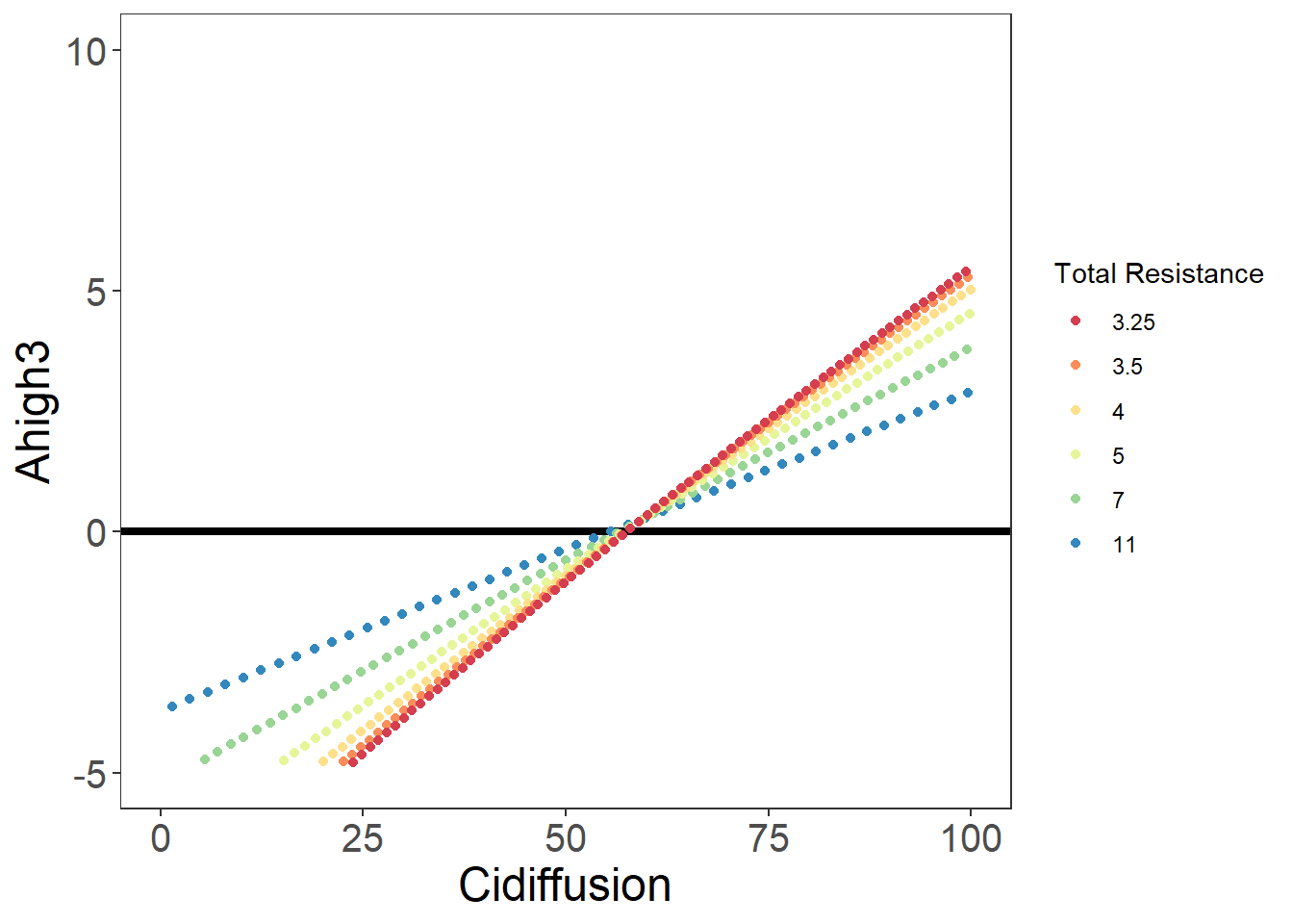

图 10.13: 不同 Ci 扩散限制下的差异

datahigh <- data[data$resistance == "11",]
graph <- ggplot(datahigh, aes(x = Cidiffusion, y = Ahigh3)) +
  geom_abline(slope=0,intercept=0,size=1.5)+
  geom_point(colour = "red")+
  geom_point(aes(x = Cidiffusion, y = Ahigh2), colour = "blue")+
  geom_point(aes(x = Cidiffusion, y = Ahigh), colour = "green")+
  labs(colour = 'Total Resistance')+
  scale_colour_brewer(palette = 'Spectral') +
  theme_bw() +
  scale_x_continuous(limits=c(0,100))+
  scale_y_continuous(limits=c(-2.5,2.5))+
  theme(
    axis.title = element_text(size = 18),
    axis.text = element_text(size = 15),
    legend.position = 'right',
    panel.grid.major = element_blank(),
    panel.grid.minor = element_blank()
  )
graph

## Warning: Removed 340 rows containing missing values (geom_point).

## Warning: Removed 340 rows containing missing values (geom_point).

## Warning: Removed 340 rows containing missing values (geom_point).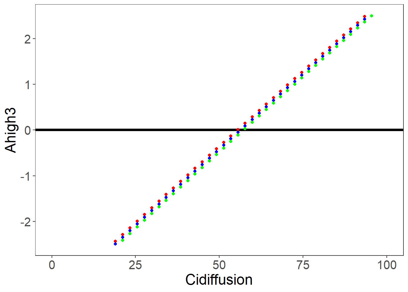

图 10.14: 不同 Ci 扩散限制下的差异（resistance = 11）

data2 <- read.csv("./data/DiffusionLimits.csv")
graph <- ggplot(data2, aes(x = TotalRes, y = Rates, colour = Scenario)) +
  geom_point()+
  scale_colour_brewer(palette = 'Spectral') +
  theme_bw() +
  theme(
    axis.title = element_text(size = 18),
    axis.text = element_text(size = 12),
    panel.grid.major = element_blank(),
    panel.grid.minor = element_blank()
  )
graph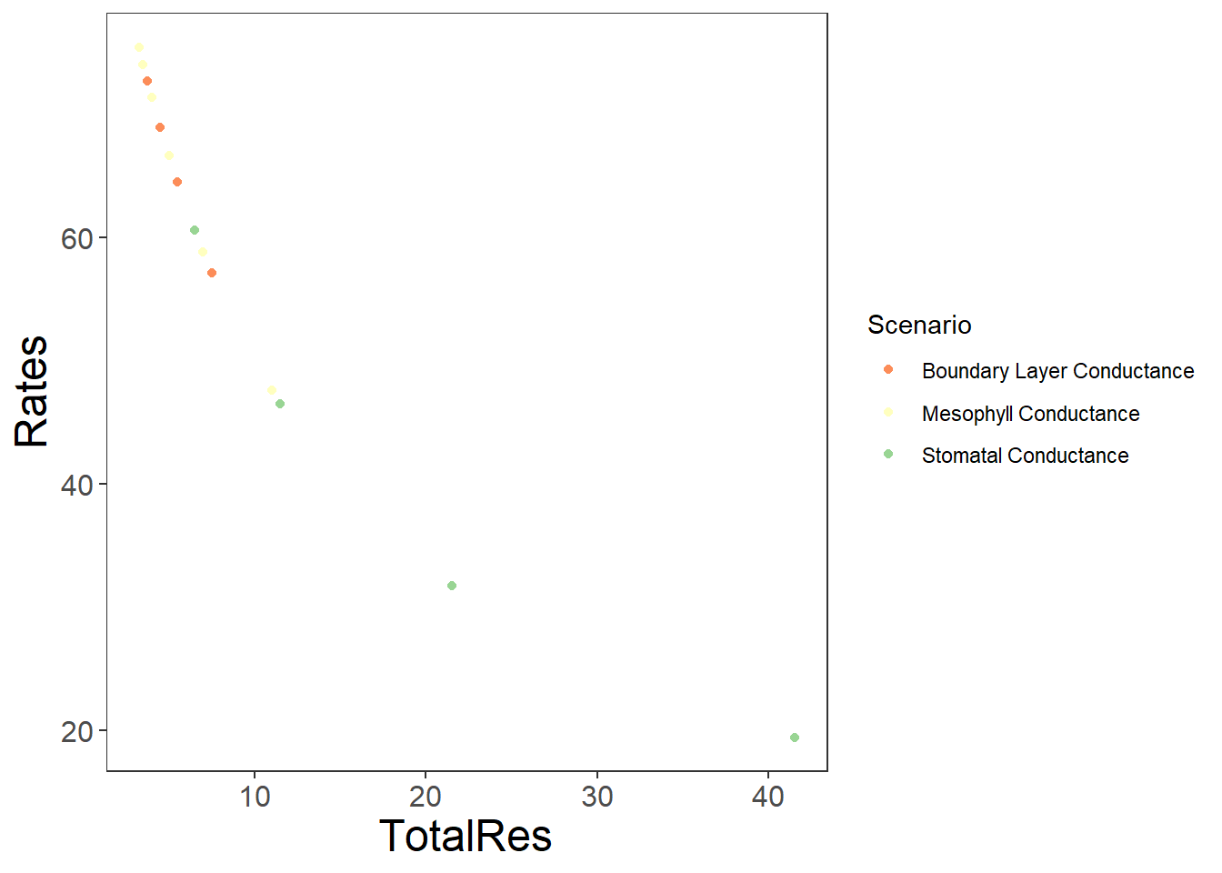

图 10.15: 不同总导度下的各个导度的速率变化

m1 <- lm(Rates ~ I(1/TotalRes)+I((1/TotalRes)^2),data=data2)
summary(m1)

## 
## Call:
## lm(formula = Rates ~ I(1/TotalRes) + I((1/TotalRes)^2), data = data2)
## 
## Residuals:
##     Min      1Q  Median      3Q     Max 
## -3.3590 -0.9844 -0.1236  0.7706  2.4510 
## 
## Coefficients:
##                   Estimate Std. Error t value Pr(>|t|)    
## (Intercept)         13.042      1.684   7.745 3.18e-06 ***
## I(1/TotalRes)      421.928     22.487  18.763 8.49e-11 ***
## I((1/TotalRes)^2) -737.690     65.500 -11.262 4.46e-08 ***
## ---
## Signif. codes:  0 '***' 0.001 '**' 0.01 '*' 0.05 '.' 0.1 ' ' 1
## 
## Residual standard error: 1.705 on 13 degrees of freedom
## Multiple R-squared:  0.9904, Adjusted R-squared:  0.9889 
## F-statistic: 668.8 on 2 and 13 DF,  p-value: 7.799e-14

ab <- predict(m1)
red <- 1/data2$TotalRes
plot(ab~red)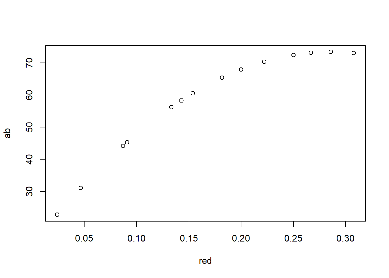

图 10.16: 不同阻力下的各个导度的速率变化预测值

10.9.1 补偿点的计算

计算补偿点，代码同前文类似，只是采用了不同导度下的数值：

data <- read.csv("./data/DiffusionLimitsACI2.csv")
#Gamma
# For Ci-based estimates, only use Ci < 100
dataCi <- data[data$Cidiffusion < 100, ]
dataCi0125 <- dataCi[dataCi$conductance == "0.125", ]
dataCi025 <- dataCi[dataCi$conductance == "0.25", ]
dataCi05 <- dataCi[dataCi$conductance == "0.5", ]
dataCi1 <- dataCi[dataCi$conductance == "1", ]
dataCi2 <- dataCi[dataCi$conductance == "2", ]
dataCi4 <- dataCi[dataCi$conductance == "4", ]
m1 <- lm(dataCi0125$Ahigh ~ dataCi0125$Cidiffusion)
summary(m1)

## 
## Call:
## lm(formula = dataCi0125$Ahigh ~ dataCi0125$Cidiffusion)
## 
## Residuals:
##       Min        1Q    Median        3Q       Max 
## -0.040649 -0.014495  0.005307  0.017054  0.021232 
## 
## Coefficients:
##                          Estimate Std. Error t value Pr(>|t|)    
## (Intercept)            -3.836e+00  4.318e-03  -888.5   <2e-16 ***
## dataCi0125$Cidiffusion  6.665e-02  7.873e-05   846.6   <2e-16 ***
## ---
## Signif. codes:  0 '***' 0.001 '**' 0.01 '*' 0.05 '.' 0.1 ' ' 1
## 
## Residual standard error: 0.01934 on 52 degrees of freedom
## Multiple R-squared:  0.9999, Adjusted R-squared:  0.9999 
## F-statistic: 7.167e+05 on 1 and 52 DF,  p-value: < 2.2e-16

Gamma0125 <- -m1$coefficients[1] / m1$coefficients[2]
m2 <- lm(dataCi025$Ahigh ~ dataCi025$Cidiffusion)
summary(m2)

## 
## Call:
## lm(formula = dataCi025$Ahigh ~ dataCi025$Cidiffusion)
## 
## Residuals:
##       Min        1Q    Median        3Q       Max 
## -0.070876 -0.025427  0.009071  0.029765  0.036593 
## 
## Coefficients:
##                         Estimate Std. Error t value Pr(>|t|)    
## (Intercept)           -5.2507346  0.0092187  -569.6   <2e-16 ***
## dataCi025$Cidiffusion  0.0904227  0.0001544   585.5   <2e-16 ***
## ---
## Signif. codes:  0 '***' 0.001 '**' 0.01 '*' 0.05 '.' 0.1 ' ' 1
## 
## Residual standard error: 0.03329 on 59 degrees of freedom
## Multiple R-squared:  0.9998, Adjusted R-squared:  0.9998 
## F-statistic: 3.428e+05 on 1 and 59 DF,  p-value: < 2.2e-16

Gamma025 <- -m2$coefficients[1] / m2$coefficients[2]
m3 <- lm(dataCi05$Ahigh ~ dataCi05$Cidiffusion)
summary(m3)

## 
## Call:
## lm(formula = dataCi05$Ahigh ~ dataCi05$Cidiffusion)
## 
## Residuals:
##      Min       1Q   Median       3Q      Max 
## -0.10435 -0.03583  0.01358  0.04311  0.05340 
## 
## Coefficients:
##                        Estimate Std. Error t value Pr(>|t|)    
## (Intercept)          -6.4051036  0.0150363    -426   <2e-16 ***
## dataCi05$Cidiffusion  0.1097686  0.0002391     459   <2e-16 ***
## ---
## Signif. codes:  0 '***' 0.001 '**' 0.01 '*' 0.05 '.' 0.1 ' ' 1
## 
## Residual standard error: 0.04851 on 65 degrees of freedom
## Multiple R-squared:  0.9997, Adjusted R-squared:  0.9997 
## F-statistic: 2.107e+05 on 1 and 65 DF,  p-value: < 2.2e-16

Gamma05 <- -m3$coefficients[1] / m3$coefficients[2]
m4 <- lm(dataCi1$Ahigh ~ dataCi1$Cidiffusion)
summary(m4)

## 
## Call:
## lm(formula = dataCi1$Ahigh ~ dataCi1$Cidiffusion)
## 
## Residuals:
##      Min       1Q   Median       3Q      Max 
## -0.13150 -0.04513  0.01709  0.05402  0.06692 
## 
## Coefficients:
##                       Estimate Std. Error t value Pr(>|t|)    
## (Intercept)         -7.1817472  0.0199135  -360.6   <2e-16 ***
## dataCi1$Cidiffusion  0.1227771  0.0003085   398.0   <2e-16 ***
## ---
## Signif. codes:  0 '***' 0.001 '**' 0.01 '*' 0.05 '.' 0.1 ' ' 1
## 
## Residual standard error: 0.06074 on 69 degrees of freedom
## Multiple R-squared:  0.9996, Adjusted R-squared:  0.9996 
## F-statistic: 1.584e+05 on 1 and 69 DF,  p-value: < 2.2e-16

Gamma1 <- -m4$coefficients[1] / m4$coefficients[2]
m5 <- lm(dataCi2$Ahigh ~ dataCi2$Cidiffusion)
summary(m5)

## 
## Call:
## lm(formula = dataCi2$Ahigh ~ dataCi2$Cidiffusion)
## 
## Residuals:
##      Min       1Q   Median       3Q      Max 
## -0.14803 -0.04874  0.01837  0.05995  0.07511 
## 
## Coefficients:
##                       Estimate Std. Error t value Pr(>|t|)    
## (Intercept)         -7.6427727  0.0230595  -331.4   <2e-16 ***
## dataCi2$Cidiffusion  0.1305083  0.0003538   368.9   <2e-16 ***
## ---
## Signif. codes:  0 '***' 0.001 '**' 0.01 '*' 0.05 '.' 0.1 ' ' 1
## 
## Residual standard error: 0.06815 on 71 degrees of freedom
## Multiple R-squared:  0.9995, Adjusted R-squared:  0.9995 
## F-statistic: 1.361e+05 on 1 and 71 DF,  p-value: < 2.2e-16

Gamma2 <- -m5$coefficients[1] / m5$coefficients[2]
m6 <- lm(dataCi4$Ahigh ~ dataCi4$Cidiffusion)
summary(m6)

## 
## Call:
## lm(formula = dataCi4$Ahigh ~ dataCi4$Cidiffusion)
## 
## Residuals:
##      Min       1Q   Median       3Q      Max 
## -0.15721 -0.05258  0.01994  0.06470  0.07968 
## 
## Coefficients:
##                       Estimate Std. Error t value Pr(>|t|)    
## (Intercept)         -7.8955772  0.0248634  -317.6   <2e-16 ***
## dataCi4$Cidiffusion  0.1347503  0.0003799   354.7   <2e-16 ***
## ---
## Signif. codes:  0 '***' 0.001 '**' 0.01 '*' 0.05 '.' 0.1 ' ' 1
## 
## Residual standard error: 0.07225 on 72 degrees of freedom
## Multiple R-squared:  0.9994, Adjusted R-squared:  0.9994 
## F-statistic: 1.258e+05 on 1 and 72 DF,  p-value: < 2.2e-16

Gamma4 <- -m6$coefficients[1] / m6$coefficients[2]

GammaCi <- c(Gamma0125, Gamma025, Gamma05, Gamma1, Gamma2, Gamma4)

10.9.2 所有图形代码

data <- read.csv("./data/PRdata.csv")
data$Ccfull <- as.numeric(data$Ccfull)
data$Delay <- as.factor(data$Delay)
cols <- gg_color_hue(6)
Panel_1A <-
  ggplot(data, aes(
    x = Cifull,
    y = Anet,
    colour = Delay,
    linetype = Delay
  )) +
  # 零水平参考线
  geom_abline(slope = 0,
              intercept = 0,
              size = 1.5) +
  #ci与A loess 方法的拟合曲线
  geom_smooth(method = "loess", se = FALSE, size = 2) +
  scale_linetype_manual(
    name = "Delay (s)",
    labels = c("0", "15", "30", "60", "120", "300"),
    values = c("solid", "longdash", "twodash", "dotdash", "dashed", "dotted")
  ) +
  ggtitle(expression(paste(
    bold("(a)"), " Modelled Photorespiratory Effect"
  ))) +
  labs(x = expression(C[i] ~ "(" * mu * mol ~ mol ^ {
    -1
  } * ")"),
  y = expression(A[net] ~ "(" * mu * mol ~ m ^ {
    -2
  } ~ s ^ {
    -1
  } * ")")) +
  labs(colour = 'Delay (s)') +
  scale_x_continuous(limits = c(0, 250)) +
  scale_y_continuous(limits = c(-5, 20)) +
  scale_colour_manual(
    values = cols,
    name = "Delay (s)",
    labels = c("0", "15", "30", "60", "120", "300")
  ) +
  theme_bw() +
  theme(
    axis.title.x = element_text(size = 20),
    axis.title.y = element_text(size = 20),
    axis.line = element_line(size = 1),
    axis.ticks = element_line(size = 1.5),
    axis.ticks.length = unit(1.5, "mm"),
    rect = element_rect(size = 2),
    axis.text.x = element_text(size = 14, color = 'black'),
    axis.text.y =
      element_text(
        size = 14,
        color = 'black',
        hjust = (1)
      ),
    legend.position = c(0.15, 0.75),
    axis.title = element_text(size = 18),
    axis.text = element_text(size = 12, color = "black"),
    panel.grid.major = element_blank(),
    panel.grid.minor = element_blank(),
    legend.text = element_text(size = 14),
    legend.title = element_text(size = 14)
  )
Panel_1A

## Warning: Removed 1029 rows containing non-finite values (stat_smooth).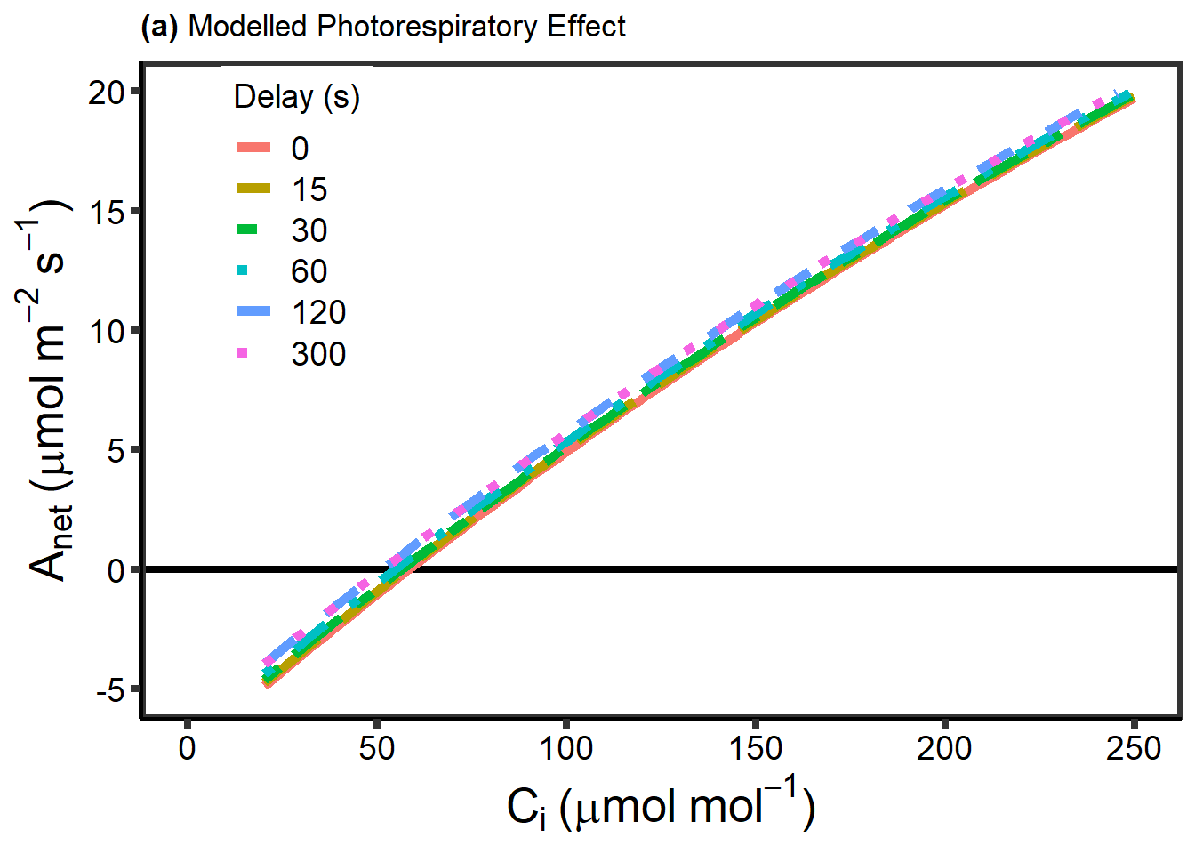

图 10.17: 不同时间滞后性的 Anet VS Ci

Panel_1A_inset <-
  ggplot(data, aes(
    x = Cifull,
    y = Anet,
    colour = Delay,
    linetype = Delay
  )) +
  geom_abline(slope = 0,
              intercept = 0,
              size = 1.5) +
  geom_smooth(method = "loess", se = FALSE, size = 2) +
  scale_linetype_manual(
    name = "Delay (s)",
    labels = c("0", "15", "30", "60", "120", "300"),
    values = c("solid", "longdash", "twodash", "dotdash", "dashed", "dotted")
  ) +
  labs(x = expression(C[i] ~ "(" * mu * mol ~ mol ^ {
    -1
  } * ")"),
  y = expression(A[net] ~ "(" * mu * mol ~ m ^ {
    -2
  } ~ s ^ {
    -1
  } * ")")) +
  labs(colour = 'Delay (s)') +
  scale_x_continuous(limits = c(45, 65)) +
  scale_y_continuous(limits = c(-1, 1), breaks = c(-1, 0, 1)) +
  scale_colour_manual(values = cols) +
  theme_bw() +
  theme(
    axis.title.x = element_blank(),
    axis.title.y = element_blank(),
    axis.line = element_line(size = 1),
    axis.ticks = element_line(size = 1.5),
    axis.ticks.length = unit(1.5, "mm"),
    rect = element_rect(size = 2),
    axis.text.x = element_text(size = 14, color = 'black'),
    axis.text.y =
      element_text(
        size = 14,
        color = 'black',
        hjust = (1)
      ),
    axis.title = element_blank(),
    axis.text = element_text(size = 12, color = "black"),
    panel.grid.major = element_blank(),
    panel.grid.minor = element_blank(),
    legend.position = 'none',
    plot.background = element_blank()
  )



cols <- gg_color_hue(6)

data <- read.csv("./data/DiffusionLimitsACI2.csv")
data$resistance <- as.factor(data$resistance)
Panel_1Db <-
  ggplot(data,
         aes(
           x = Cidiffusion,
           y = Ahigh,
           colour = resistance,
           linetype = resistance
         )) +
  geom_abline(slope = 0,
              intercept = 0,
              size = 1.5) +
  geom_smooth(method = "loess", se = FALSE, size = 2) +
  scale_linetype_manual(
    name = "Total Resistance",
    labels = c("3.25", "3.5", "4", "5", "7", "11"),
    values = c("solid", "longdash", "twodash", "dotdash", "dashed", "dotted")
  ) +
  ggtitle(expression(paste(bold("(d)"), " Modelled Resistance Effect"))) +
  scale_color_manual(
    values = cols,
    name = "Total Resistance",
    labels = c("3.25", "3.5", "4", "5", "7", "11")
  ) +
  theme_bw() +
  labs(x = expression(paste(C[i] ~ "(" * mu * mol ~ mol ^ {
    -1
  } * ")")), y = expression(paste(A[net] ~ "(" * mu * mol ~ m ^ {
    -2
  } ~ s ^ {
    -1
  } * ")"))) +
  scale_x_continuous(limits = c(0, 250)) +
  scale_y_continuous(limits = c(-5, 20)) +
  theme(
    axis.title.x = element_text(size = 20),
    axis.title.y = element_text(size = 20),
    axis.line = element_line(size = 1),
    axis.ticks = element_line(size = 1.5),
    axis.ticks.length = unit(1.5, "mm"),
    rect = element_rect(size = 2),
    axis.text.x = element_text(size = 14, color = 'black'),
    axis.text.y =
      element_text(
        size = 14,
        color = 'black',
        hjust = (1)
      ),
    legend.position = c(0.22, 0.75),
    axis.title = element_text(size = 18),
    axis.text = element_text(size = 12, color = "black"),
    panel.grid.major = element_blank(),
    panel.grid.minor = element_blank(),
    legend.text = element_text(size = 14),
    legend.title = element_text(size = 14)
  )
Panel_1Db

## Warning: Removed 1159 rows containing non-finite values (stat_smooth).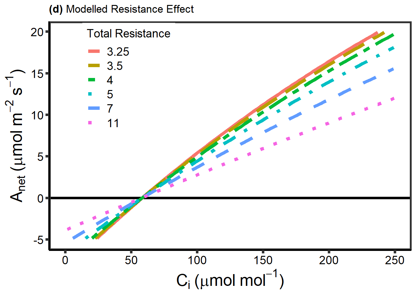

图 10.18: 不同总阻力下的 Anet VS Ci

data <- read.csv("./data/DiffusionLimitsACI2.csv")
data$resistance <- as.factor(data$resistance)
data <- data[data$resistance == "11",]
resistance <- rep(data$resistance, 3)
Cidiffusion <- rep(data$Cidffusion, 3)
A <- c(data$Ahigh, data$Ahigh2, data$Ahigh3)
Rate <-
  c(rep(100, length(data$Ahigh)), rep(200, length(data$Ahigh2)), rep(300, length(data$Ahigh3)))
data3 <- rbind(data, data, data)
data3$A <- c(data$Ahigh, data$Ahigh2, data$Ahigh3)
data3$Rate <-
  as.factor(c(rep(100, length(data$Ahigh)), rep(200, length(data$Ahigh2)), rep(300, length(data$Ahigh3))))
Panel_1Dbinset <-
  ggplot(data3, aes(
    x = Cidiffusion,
    y = A,
    colour = Rate,
    linetype = Rate
  )) +
  geom_abline(slope = 0,
              intercept = 0,
              size = 1.5) +
  geom_smooth(method = "loess", se = FALSE, size = 2) +
  scale_linetype_manual(
    name = "Rate",
    labels = c("100", "200", "300"),
    values = c("solid", "longdash", "twodash")
  ) +
  scale_color_manual(
    values = cols,
    name = "Rate",
    labels = c("100", "200", "300")
  ) +
  theme_bw() +
  labs(x = expression(paste(C[i] ~ "(" * mu * mol ~ mol ^ {
    -1
  } * ")")), y = expression(paste(A[net] ~ "(" * mu * mol ~ m ^ {
    -2
  } ~ s ^ {
    -1
  } * ")"))) +
  scale_x_continuous(limits = c(45, 65)) +
  scale_y_continuous(limits = c(-1, 1), breaks = c(-1, 0, 1)) +
  theme(
    axis.title.x = element_blank(),
    axis.title.y = element_blank(),
    axis.line = element_line(size = 1),
    axis.ticks = element_line(size = 1.5),
    axis.ticks.length = unit(1.5, "mm"),
    rect = element_rect(size = 2),
    axis.text.x = element_text(size = 14, color = 'black'),
    axis.text.y =
      element_text(
        size = 14,
        color = 'black',
        hjust = (1)
      ),
    legend.position = c(0.22, 0.75),
    axis.title = element_text(size = 18),
    axis.text = element_text(size = 12, color = "black"),
    panel.grid.major = element_blank(),
    panel.grid.minor = element_blank(),
    plot.background = element_blank(),
    legend.text = element_text(size = 12),
    legend.key = element_blank(),
    legend.title = element_blank(),
    legend.background = element_blank()
  )
Panel_1Dbinset

## Warning: Removed 1101 rows containing non-finite values (stat_smooth).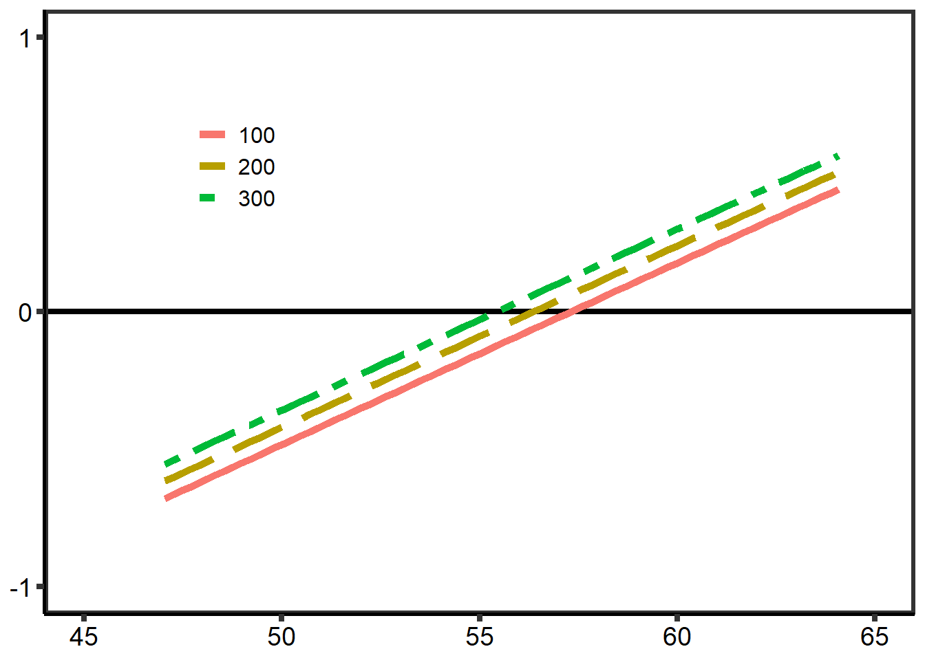

图 10.19: 不同导度下的 A VS Ci

data2 <- read.csv("./data/DiffusionLimits.csv")
data2$Conductance <-
  revalue(
    data2$Scenario,
    c(
      "Boundary Layer Conductance" = "Boundary Layer",
      "Mesophyll Conductance" = "Mesophyll",
      "Stomatal Conductance" = "Stomatal"
    )
  )
cols <- gg_color_hue(3)

Panel_1E <-
  ggplot(data2, aes(x = TotalRes, y = Rates, colour = Conductance)) +
  geom_point(size = 4) +
  ggtitle(expression(paste(bold("(e)"), " Modelled Resistance Effect"))) +
  labs(x = expression(paste(r[total] * " (s" ~ m ^ {
    2
  } ~ mol ^ {
    -1
  } * ")")), 
  y = expression(paste(C[c] * " Ramp Rate (" * mu * mol ~ mol ^
                                    {
                                      -1
                                    } ~ min ^ {
                                      -1
                                    } * ")"))) +
  scale_x_continuous(limits = c(0, 50)) +
  scale_y_continuous(limits = c(0, 80)) +
  scale_color_manual(
    values = cols,
    name = "Manipulated Resistance",
    labels = c("Boundary Layer", "Mesophyll", "Stomatal")
  ) +
  theme_bw() +
  theme(
    axis.title.x = element_text(size = 20),
    axis.title.y = element_text(size = 20),
    axis.line = element_line(size = 1),
    axis.ticks = element_line(size = 1.5),
    axis.ticks.length = unit(1.5, "mm"),
    rect = element_rect(size = 2),
    axis.text.x = element_text(size = 14, color = 'black'),
    axis.text.y =
      element_text(
        size = 14,
        color = 'black',
        hjust = (1)
      ),
    legend.position = c(0.70, 0.84),
    axis.title = element_text(size = 18),
    axis.text = element_text(size = 12, color = "black"),
    panel.grid.major = element_blank(),
    panel.grid.minor = element_blank(),
    legend.text = element_text(size = 14),
    legend.title = element_text(size = 14)
  )
Panel_1E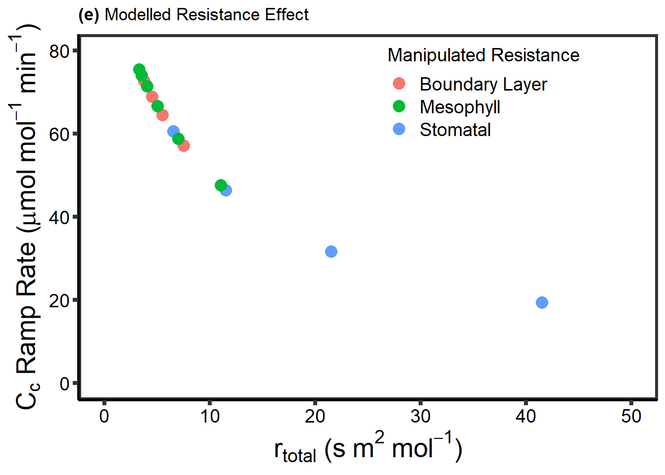

图 10.20: 不同总导度下的各个导度的变化

data <- read.csv("./data/RASdata.csv")
data$Ccfull <- as.numeric(data$Ccfull)
data$Deactivation <- as.factor(data$Deactivation)
print(levels(data$Deactivation))

## [1] "High"   "Low"    "Medium" "None"

data$Deactivation <-
  factor(data$Deactivation, levels(data$Deactivation)[c(4, 2, 3, 1)])
FigS1 <-
  ggplot(data,
         aes(
           x = Cifull,
           y = Anet,
           colour = Deactivation,
           linetype = Deactivation
         )) +
  geom_smooth(method = "loess", se = FALSE, size = 2) +
  scale_linetype_manual(
    name = "Deactivation",
    labels = c("None", "Low", "Medium", "High"),
    values = c("solid", "longdash", "dashed", "dotted")
  ) +
  labs(x = expression(C[i] ~ "(" * mu * mol ~ mol ^ {
    -1
  } * ")"),
  y = expression(A[net] ~ "(" * mu * mol ~ m ^ {
    -2
  } ~ s ^ {
    -1
  } * ")")) +
  labs(colour = 'Deactivation') +
  scale_x_continuous(limits = c(25, 100),
                     breaks = c(25, 40, 55, 70, 85, 100)) +
  scale_y_continuous(limits = c(-5, 5)) +
  geom_hline(yintercept = 0, size = 1.5) +
  theme_bw() +
  theme(
    axis.title.x = element_text(size = 20),
    axis.title.y = element_text(size = 20),
    axis.line = element_line(size = 1),
    axis.ticks = element_line(size = 1.5),
    axis.ticks.length = unit(1.5, "mm"),
    rect = element_rect(size = 2),
    axis.text.x = element_text(size = 14, color = 'black'),
    axis.text.y =
      element_text(
        size = 14,
        color = 'black',
        hjust = (1)
      ),
    legend.position = c(0.8, 0.2),
    legend.text = element_text(size = 16),
    legend.title = element_text(size = 16),
    panel.grid.major = element_blank(),
    panel.grid.minor = element_blank()
  )
FigS1

## Warning: Removed 1230 rows containing non-finite values (stat_smooth).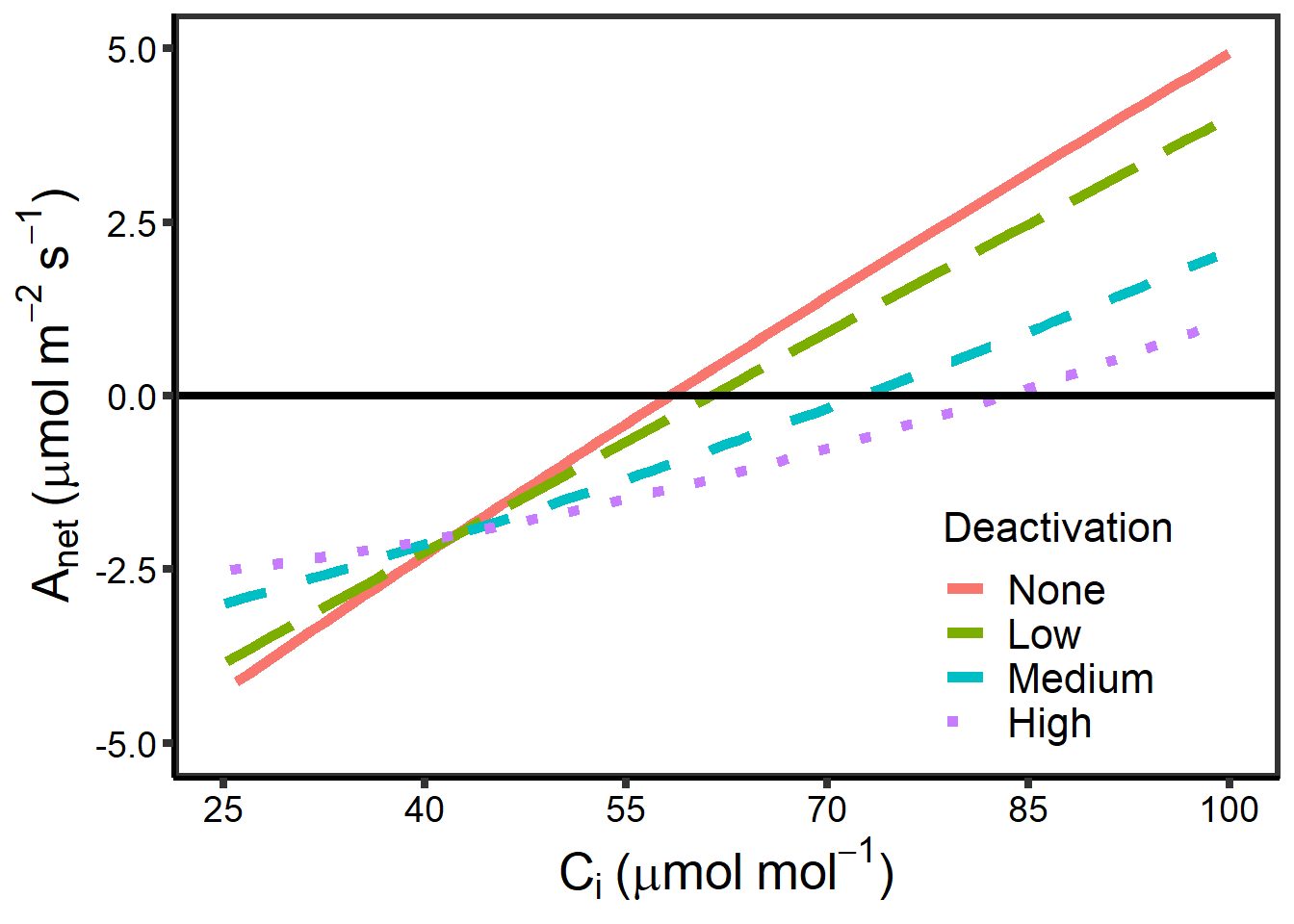

图 10.21: Rubisco不同失活程度下的下 A VS Ci

10.10 LI-6800 荧光数据分析

LI-6800 能够直接提供基本的叶绿素荧光参数，其他参数均可通过这些基本的参数进行计算，计算也较简单，在此不赘述，需要注意的是快相荧光部分的数据，因为分析 ojip 数据的模型有很多，很多都需要复杂的计算，在此我们先将其中较为简单的 jip test 数据分析进行介绍。

10.10.1 jip test 的实现

LI-6800 增加了 ojip 曲线测量功能，本功能主要是针对测量数据的 jip test 的实现。

10.10.2 `jiptest` 软件包安装

请在 github 安装，有可能需要安装 remotes

install.packages("remotes")

然后安装：

install_github("zhujiedong/jiptest")

如果因为网络原因失败，可以转战 gitee:

install_git('https://gitee.com/zhu_jie_dong/jiptest')

10.10.3 `read_files` 及 `read_dcfiles` 函数

read_files 用于批量读取所有调制光测量数据，方便用于其他的数据分析。函数要求所有数据必须是 xlsx 格式，并且所有测量数据都保存在同一文件夹内。，如有其他文件或测量数据则会报错。 read_dcfiles 用于批量读取所有连续光测量数据，其他与 read_dcfiles 相同。例如我放在了 data文件夹下的 ojip 文件夹内，有五个数据文件。

函数仅有一个参数，即保存数据文件夹的路径，使用如下：

library(jiptest)
jip_data<- read_files("data/ojip")

jip_dcdata <- read_dcfiles("./data/ojip")

调制光的信号前 10 行数据：

表 10.1: jiptest 批量导入数据后的样式
SECS	FLUOR	NORM_FLUOR	SOURCE
6.10e-06	621	0.0005027	INDUCTION-4188-20201116-10_53_39
1.01e-05	620	0.0000000	INDUCTION-4188-20201116-10_53_39
1.42e-05	649	0.0145781	INDUCTION-4188-20201116-10_53_39
1.80e-05	629	0.0045242	INDUCTION-4188-20201116-10_53_39
2.21e-05	674	0.0271455	INDUCTION-4188-20201116-10_53_39
2.61e-05	736	0.0583126	INDUCTION-4188-20201116-10_53_39

连续光的信号前 10 行数据：

表 10.2: jiptest DC 数据批量导入数据后的样式
SECS	FLUOR	NORM_FLUOR	SOURCE
6.10e-06	98161	0.0000000	INDUCTION-4188-20201116-10_53_39
1.01e-05	100331	0.0071347	INDUCTION-4188-20201116-10_53_39
1.42e-05	102577	0.0145193	INDUCTION-4188-20201116-10_53_39
1.80e-05	104849	0.0219894	INDUCTION-4188-20201116-10_53_39
2.21e-05	107214	0.0297652	INDUCTION-4188-20201116-10_53_39
2.61e-05	109624	0.0376890	INDUCTION-4188-20201116-10_53_39

注：NORM_FLUOR 是标准化后的荧光信号数据，其中标准化采用的方式是 Stirbet and Govindjee (2012) 所采用的：\(F = \frac{F_t - F_o}{F_m - F_o}\)，而曲线上部的面积则采用 Stirbet and Govindjee (2011) 的方式进行标准化，以方便不同叶片之间的比较，具体为 \(area = \frac{area}{F_m - F_o}\)

10.10.4 `jip_test` 及 `jip_dctest` 函数

jiptest 是 jiptest 的核心函数，用于所有数据的 jiptest 分析，函数仅包一个参数，测量数据的保存文件夹路径。 jip_dctest 与 jip_test 相似，用于连续光测量数据的分析。

actest <- jip_test("./data/ojip")

dctest <- jip_dctest("./data/ojip")

可以看出，对于标准化之后的参数，二者基本一致，原始信号则无法一致，因为连续光信号强度更高（所以数据的比较要在相同的测量光内进行）：

调制光信号的计算参数：

表 10.3: jiptest 输出的计算参数
parameters	data_file1	data_file2	data_file3	data_file4	data_file5
Fo	620.000	887.000	849.000	981.000	914.000
Fm	2609.280	4649.520	3714.270	4225.240	3754.270
F300	1593.200	2181.400	1798.600	2067.800	2537.200
FJ	1722.900	2594.300	2104.600	2456.800	2569.000
FI	2268.950	4443.110	3547.110	4009.220	3556.530
Tfmax	159.998	256.016	316.016	272.016	200.016

连续光信号计算参数：

表 10.4: jiptest DC 数据输出的计算参数
parameters	data_file1	data_file2	data_file3	data_file4	data_file5
Fo	98161.000	154000.000	133191.000	156664.000	153589.000
Fm	402308.000	713839.000	560610.000	647660.000	584839.000
F300	246753.000	338091.000	275476.800	322859.200	388110.400
FJ	267827.000	400744.000	320245.000	376885.000	406671.000
FI	349985.000	681505.000	534314.000	614590.000	552253.000
Tfmax	171.998	276.016	300.016	288.016	212.016

计算参数见表 10.3 及 10.4，考虑到排版，仅显示部分内容。若需要将数据导出，可以使用相关命令，如：

# export the results of jiptest to a csv file
write.csv(actest, "d:/data/jip_resluts.csv")
write.csv(dctest, "d:/data/dcjip_resluts.csv")

10.10.5 图像查看函数

之前的预览方式已经彻底从代码中删除，不在提供。如果仅仅是简单查看结果，那么我们直接用默认参数就好，作图的数据是之前导入的数据文件：

默认使用标准化的荧光信号（也就是除以最大值，标准化到 0~1 之间，LI-6800 在 1.4 之后的版本也提供了仪器上查看的界面）。

10.10.5.1 默认图形的方式

默认调制光图形

plot(jip_data)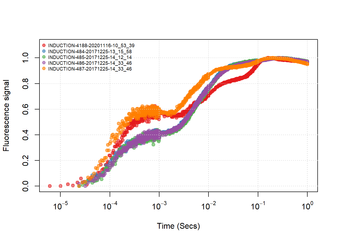

图 10.22: 默认调制光图形查看

默认连续光图形

plot(jip_dcdata)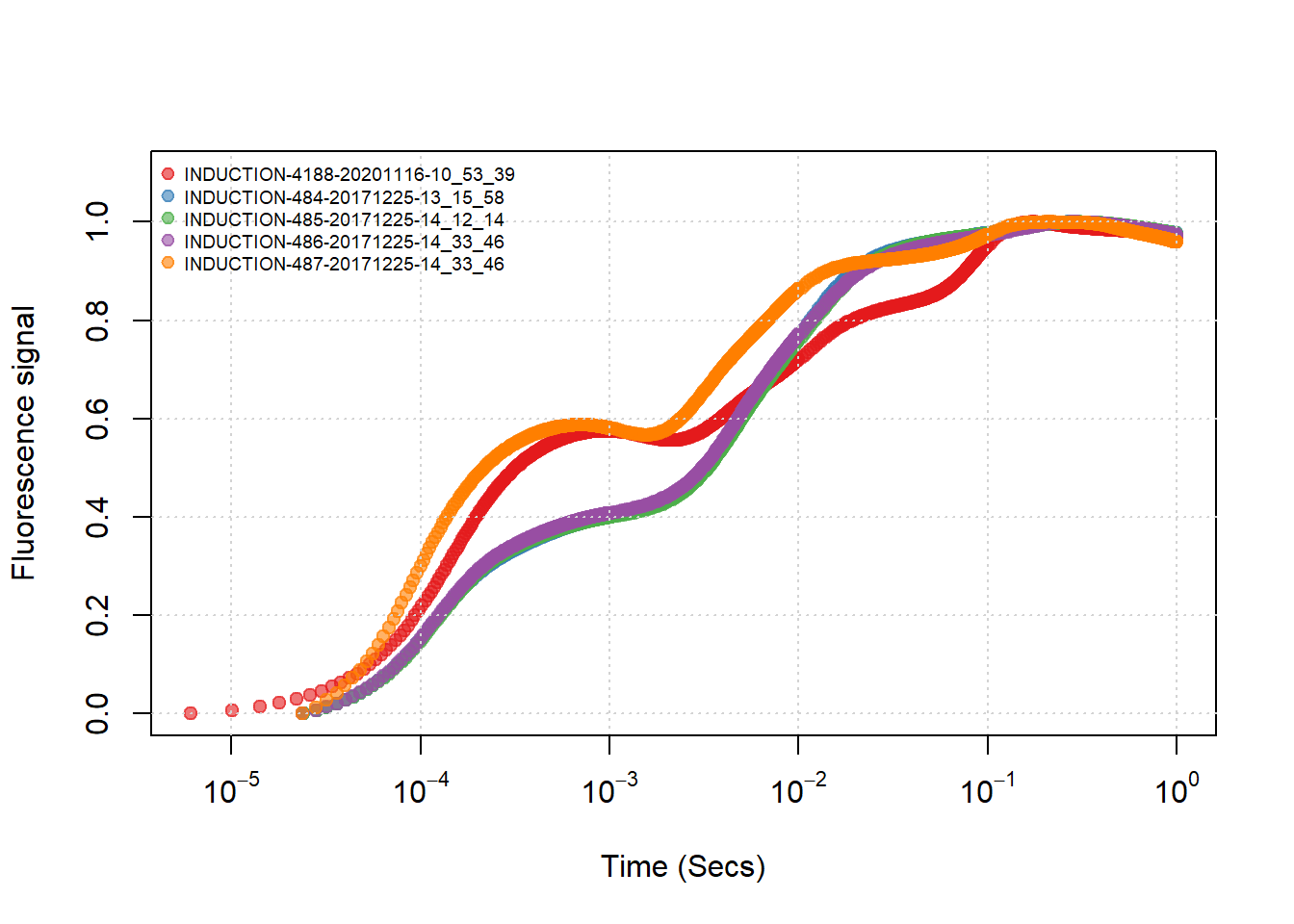

图 10.23: 默认连续光图形查看

默认图形，仅仅查看结果是可以的，当然有些情况下需要进行调整才方便做展示用。

10.10.5.2 定制化图形的方式

这个是这次改动的重点之一，例如都使用原始信号分别做上面两幅图：

定制调制光图形

这里使用原始荧光信号，然后更改图例颜色等，主要是 add_leg = FALSE 不增加默认的图例，以及 normalized = FALSE 不使用信号标准化。其他请参考帮助 ?plot.jip。我简单写了一下帮助文档，大家应该基本能看明白，我实在没时间。

cls <- palette.colors(n = 5,  "set 2", alpha = 0.8)
plot(jip_data,
     ylab = 'Normalized fluorescence signals',
     add_leg = FALSE,
     def_pch = 14:18,
     col = cls,
     main = "Demodulated signals", normalized = FALSE)

legend(
  "topleft",
  unique(jip_data$SOURCE),
  col = cls,
  pch = 14:18,
  cex = 0.6,
  pt.cex = 1.2,
  bty = "n")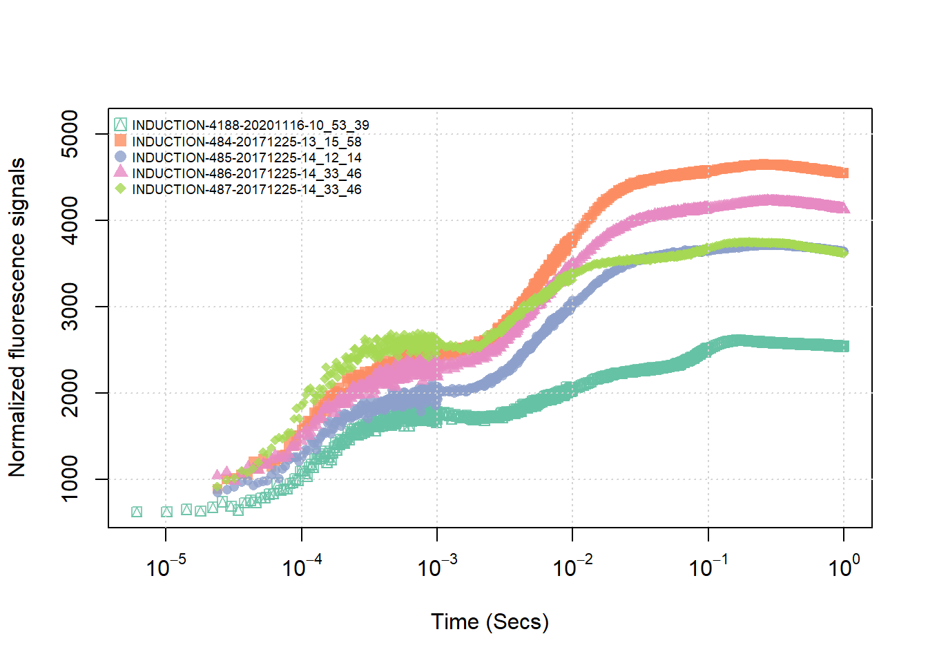

图 10.24: 定制调制光图形示例

定制连续光图形

连续光图形，只改了两个地方，图例的位置以及不显示标准化的数据。

plot(jip_dcdata, legend_pos = "bottomright", normalized = FALSE)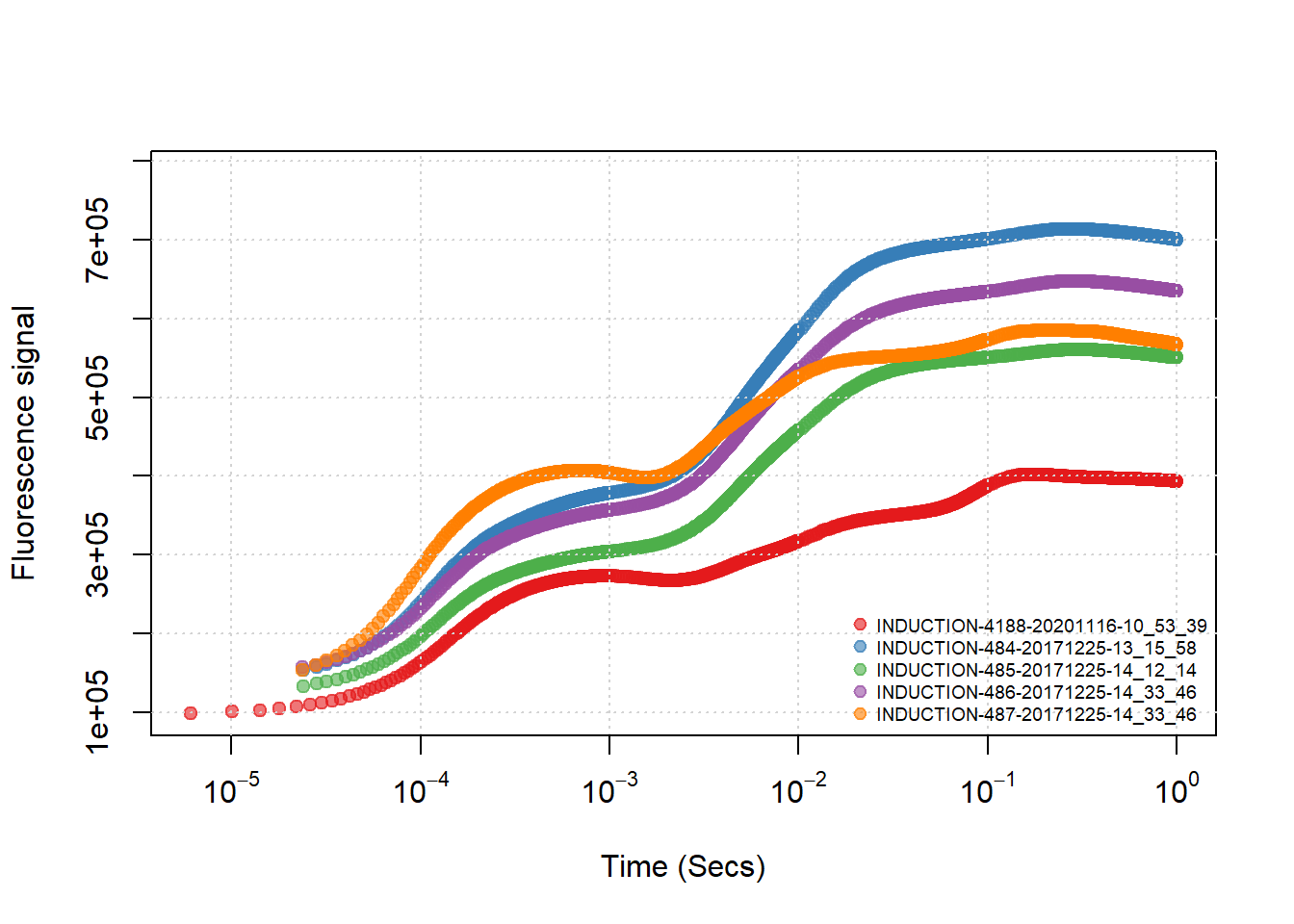

图 10.25: 定制连续光图形示例

关于标准化和非标准化图形差异大的问题，这个比较简单，原始信号比较低的那条线，是不同物种的不同叶片，所以不具备比较价值，我只是数据测试。

建议在开始分析数据前，使用如上方式作图查看数据质量，若使用调制光数据测量的荧光信号太弱，数据点太散，则可以使用连续光测量信号进行分析，对于归一化的荧光参数，二者几乎无差别，当然避免陷入被动的最好方式还是最开始测量时注意检查数据质量

参考文献

Coursolle, Carole, Guillaume O. Prud’homme, Manuel Lamothe1, and Nathalie Isabel1. 2019. “Measuring Rapid a–Ci Curves in Boreal Conifers: Black Spruce and Balsam Fir.” Frontiers in Plant Science. https://doi.org/10.3389/fpls.2019.01276.

Joseph R., Stinziano, Adamson Rachael K., and Hanson David T. 2019. “Using Multirate Rapid ACi Curves as a Tool to Explore New Questions in the Photosynthetic Physiology of Plants.” New Phytologist. https://doi.org/10.1111/nph.15657.

Stinziano, J. R., P. B. Morgan, D. J. Lynch, A. J. Saathoff, D. K. Mcdermitt, and D. T. Hanson. 2017. “The Rapid a-Ci Response: Photosynthesis in the Phenomic Era.” Plant Cell & Environment 40.

Stinziano, Joseph R, Dayle K Mcdermitt, Douglas J Lynch, Aaron J Saathoff, Patrick B Morgan, and David T Hanson. 2018. “The Rapid a/Ci Response: A Guide to Best Practices.” New Phytologist.

Stirbet, Alexandrina, and Govindjee. 2011. “On the Relation Between the Kautsky Effect (Chlorophyll a Fluorescence Induction) and Photosystem II: Basics and Applications of the OJIP Fluorescence Transient.” Journal of Photochemistry and Photobiology B: Biology, Special Issue on Recent Progress in the Studies of Structure and Function of Photosystem II, 104 (1): 236–57. https://doi.org/10.1016/j.jphotobiol.2010.12.010.

Stirbet, Alexandrina, and Govindjee. 2012. “Chlorophyll a Fluorescence Induction: A Personal Perspective of the Thermal Phase, the J–I–P Rise.” Photosynthesis Research 113 (1): 15–61. https://doi.org/10.1007/s11120-012-9754-5.