第 8 章光响应曲线的拟合

光响应曲线模型有很多，主要分为四大类，直角双曲线，非直角双曲线，指数以及直角双曲线修正模型，我们分别对这四类进行阐述。

8.1 直角双曲线模型

Baly (1935) 提出了直角双曲线模型，它的表达式为：

\[\begin{equation} P_{n} = \frac{\alpha I\ P_{nmax}}{\alpha I + P_{nmax}}- R_{d} \tag{8.1} \end{equation}\]

其中，\(P_{n}\) 为净光合速率；
I 为光强；
\(\alpha\) 为光响应曲线在光强为 0 时的斜率，即光响应曲线的初始斜率，也称之为初始量子效率；
\(P_{nmax}\) 为最大净光合速率；
\(R_{d}\)：为暗呼吸速率。

对 (8.1) 求导可知其导数大于 0，也就是直角双曲线是一个没有极值的渐近线，因此，无法由 (8.1) 求得最大光合速率的饱和光强¹²。

因此就需要使用弱光条件下 (\(\leq\) 200 \(\mu mol\cdot m^{-2}\cdot s^{-1}\)) 的数据得到表观量子效率（apparent quantum efficiency，AQE），利用非线性最小二乘法估算 P\(_{nmax}\) ，然后利用 ZiPiao (2010) 的式 (8.2) 求解 \(I_{sat}\)，

\[\begin{equation} P_{nmax}= AQE \times I_{sat} - R_{d} \tag{8.2} \end{equation}\]

但此方法测得的光饱和点远小于实测值，我们采用 0.7P\(_{nmax}\) Zhang, Shen, and Song (2009)、0.9P\(_{nmax}\) Huang et al. (2009)、或其他设定的值来的来估算\(I_{sat}\)。

8.1.1 直角双曲线模型的实现

若没有安装 minpack.lm, 则需要首先：

install.packages("minpack.lm")

具体实现过程如下：

# 调用非线性拟合包minpack.lm，也可以直接使用nls
library(minpack.lm)
# 读取数据，同fitaci数据格式
lrc <- read.csv("./data/lrc.csv")
lrc <- subset(lrc, Obs > 0)

# 光响应曲线没有太多参数，
# 直接调出相应的光强和光合速率
# 方便后面调用
lrc_Q <- lrc$PARi
lrc_A <- lrc$Photo 

# 采用非线性拟合进行数据的拟合
lrcnls <- nlsLM(lrc_A ~ (alpha * lrc_Q * Am) * 
                (1/(alpha * lrc_Q + Am)) - Rd,  
              start=list(Am=(max(lrc_A)-min(lrc_A)),
              alpha=0.05,Rd=-min(lrc_A))
)
fitlrc_rec <- summary(lrcnls)

# 补偿点时净光合速率为0，
# 据此利用uniroot求解方程的根
Ic <- function(Ic){(fitlrc_rec$coef[2,1] * Ic *
    fitlrc_rec$coef[1,1]) * (1/(fitlrc_rec$coef[2,1] * 
    Ic + fitlrc_rec$coef[1,1])) - fitlrc_rec$coef[3,1] 
}

uniroot(Ic, c(0,50))$root

## [1] 3.650053

# 根据饱和点定义，0.75最大光合速率为饱和点，
# 也可以是其他比例
# 据此利用uniroot求解方程的根

Isat <- function(Isat){(fitlrc_rec$coef[2,1] * 
        Isat * fitlrc_rec$coef[1,1]) * 
    (1/(fitlrc_rec$coef[2,1] * Isat + 
          fitlrc_rec$coef[1,1])) - fitlrc_rec$coef[3,1] -
    0.75 * fitlrc_rec$coef[1,1]
}
# 求值区间根据具体实验确定

uniroot(Isat, c(0,2500))$root

## [1] 700.0946

# 使用ggplot2进行作图并拟合曲线
library(ggplot2)

light <- data.frame(lrc_Q = lrc$PARi, lrc_A = lrc$Photo)

p <- ggplot(light, aes(x = lrc_Q, y = lrc_A))

p1 <- p + geom_point(shape = 16, size = 3, color = "green") + 
  geom_smooth(method="nls", formula = y ~ (alpha * x * Am) * 
  (1/(alpha * x + Am)) - Rd, se = FALSE,
  method.args = 
  list(start = c(Am=(max(lrc_A)-min(lrc_A)),
  alpha=0.05,Rd=-min(lrc_A)), 
  aes(x =lrc_Q, y = lrc_A, color='blue', size = 1.2))
  ) +
  labs(y=expression(paste("photosynthetic rate  ", 
       "(", mu, mol%.%m^-2%.%s^-1, ")")), 
       x=expression(paste("PAR ", 
       "(", mu, mol%.%m^-2%.%s^-1, ")"))
       )


# 自定义坐标轴
p1 + scale_x_continuous(breaks = seq(0, 2100, by = 200)) +  
  scale_y_continuous(breaks= round(light$lrc_A)) +
  theme(axis.text.x  = element_text(
    size = 10, angle=30, vjust=0.5), 
    axis.text.y = element_text(size = 10),
    axis.title.x = element_text(size = 12, face = 'bold'),
    axis.title.y = element_text(size = 12, face = 'bold')
  )

图 8.1: 直角双曲线模型拟合

代码目的见注释，其实现过程主要分三步：

数据的导入，这与之前相同，具体格式方法参考前文 \(\ref{fitaci}\)。
光响应曲线的拟合，使用到了非线性模型 nlsLM，也可以使用 nls，具体实现方法请查看参考文档。
求饱和点和补偿点，补偿点的计算根据其定义，净光合速率为 0，求解模型在一定区间的根来计算，而饱和点则较为麻烦，若使用式 (8.2) 计算，那么饱和点远远低于我们实际需求的，因此，我们使用了 0.75P\(_{nmax}\) 来计算，求得目标区间的根。当然也可以采用其他比例来作为饱和点光合速率。

表 8.1: 直角双曲线计算参数
	Estimate	Std. Error	t value	Pr(>\|t\|)
Am	16.6721752	0.1522849	109.480151	0.0000000
alpha	0.0783312	0.0026774	29.256870	0.0000000
Rd	0.2810926	0.0789338	3.561117	0.0051716

最终的数据拟结果如图 8.1 所示，拟合的参数及结果见表 8.1。

8.2 非直角双曲线模型

Thornley (1976) 提出了非直角双曲线模型，它的表达式为：

\[\begin{equation} P_{n} = \frac{\alpha I + P_{nmax} \sqrt{(\alpha I + P_{nmax})^{2} - 4 \theta \alpha I P_{nmax}}}{2 \theta} - R_{d} \tag{8.3} \end{equation}\]

其中，\(\theta\) 为表示曲线弯曲程度的曲角参数，取值为\(0\leq \theta \leq 1\)。其他参数意义同式 (8.1)。同样如同直角双曲线模型，式仍然没有极值，无法求得 \(I_{sat}\)，可以仍然参考直角双曲线模型的方式进行计算。

8.2.1 非直角双曲线模型的实现

library(minpack.lm)

# 读取数据，同fitaci数据格式
lrc <- read.csv("./data/lrc.csv")
lrc <- subset(lrc, Obs > 0)

# 光响应曲线没有太多参数，
# 直接调出相应的光强和光合速率
# 方便后面调用
lrc_Q <- lrc$PARi
lrc_A <- lrc$Photo 

# 非直角双曲线模型的拟合
lrcnls <- nlsLM(lrc_A ~ 
                (1/(2*theta))*
                (alpha*lrc_Q+Am-sqrt((alpha*lrc_Q+Am)^2 - 
                4*alpha*theta*Am*lrc_Q))- Rd,
                start=list(Am=(max(lrc_A)-min(lrc_A)),
                alpha=0.05,Rd=-min(lrc_A),theta=1)) 

fitlrc_nrec <- summary(lrcnls)

# 光补偿点
Ic <- function(Ic){
  (1/(2 * fitlrc_nrec$coef[4,1])) * 
    (fitlrc_nrec$coef[2,1] * Ic + fitlrc_nrec$coef[1,1] - 
    sqrt((fitlrc_nrec$coef[2,1] * Ic + fitlrc_nrec$coef[1,1]
    )^2 -  4 * fitlrc_nrec$coef[2,1] * 
    fitlrc_nrec$coef[4,1] * fitlrc_nrec$coef[1,1] * Ic)) -
    fitlrc_nrec$coef[3,1]
}

uniroot(Ic, c(0,50))$root

## [1] 2.234292

# 光饱和点
Isat <- function(Isat){
  (1/(2 * fitlrc_nrec$coef[4,1])) * (fitlrc_nrec$coef[2,1] * 
  Isat + fitlrc_nrec$coef[1,1] - sqrt(
  (fitlrc_nrec$coef[2,1] * Isat +fitlrc_nrec$coef[1,1])^2 - 
  4*fitlrc_nrec$coef[2,1] * fitlrc_nrec$coef[4,1] * 
  fitlrc_nrec$coef[1,1] * Isat)) - 
  fitlrc_nrec$coef[3,1] - (0.9*fitlrc_nrec$coef[1,1])}

uniroot(Isat, c(0,2000))$root

## [1] 1596.286

# 使用ggplot2进行作图并拟合曲线
library(ggplot2)
light <- data.frame(lrc_Q = lrc$PARi, lrc_A = lrc$Photo)

p <- ggplot(light, aes(x = lrc_Q, y = lrc_A))

p1 <- p + geom_point(shape = 16, size = 3, color = "green") + 
  geom_smooth(method="nls", formula = y ~ 
  (1/(2*theta))*(alpha*x+Am-sqrt((alpha*x+Am)^2 - 
   4*alpha*theta*Am*x))- Rd, se = FALSE,
   method.args = list(start = c(Am=(max(lrc_A)-min(lrc_A)), 
   alpha=0.05, Rd=-min(lrc_A), theta=1), 
    aes(x =lrc_Q, y = lrc_A, color='blue', size = 1.2))
) +
  labs(y=expression(paste("photosynthetic rate  ", 
          "(", mu, mol%.%m^-2%.%s^-1, ")")), 
       x=expression(paste("PAR ", 
           "(", mu, mol%.%m^-2%.%s^-1, ")")))

# 自定义坐标轴
p1 + scale_x_continuous(breaks = seq(0, 2100, by = 200)) +  
  scale_y_continuous(breaks= round(light$lrc_A)) +
   theme(axis.text.x  = element_text(
    size = 10, angle=30, vjust=0.5), 
    axis.text.y = element_text(size = 10),
    axis.title.x = element_text(size = 12, face = 'bold'),
    axis.title.y = element_text(size = 12, face = 'bold')
  )

图 8.2: 非直角双曲线模型拟合

表 8.2: 非直角双曲线计算参数
	Estimate	Std. Error	t value	Pr(>\|t\|)
Am	15.8017296	0.1513064	104.435285	0.0000000
alpha	0.0658067	0.0020216	32.551422	0.0000000
Rd	0.1461717	0.0420800	3.473659	0.0070082
theta	0.3700908	0.0493403	7.500783	0.0000369

最终的数据拟结果如图 8.2 所示，拟合的参数及结果见表 8.2。单纯从作图来看，本例数据使用非直角双曲线与散点图重合程度更高。

8.3 指数模型

光合指数模型较多，我们此处使用的指数函数的模型 Prado and Moraes (1997)，其表达式为：

\[\begin{equation} P_{n} = P_{nmax}[1 - e^{-b(I-I_{C})}] \tag{8.4} \end{equation}\]

其中，\(I_{c}\) 为光补偿点，\(e\) 为自然对数的底，b为常数，其他参数意义同 (8.4)。同样，该方程仍然是没有极值的函数，但我们可以直接求得光补偿点。

8.3.1 指数模型的实现

library(minpack.lm)

# 读取数据，同fitaci数据格式
lrc <- read.csv("./data/lrc.csv")
lrc <- subset(lrc, Obs > 0)

# 光响应曲线没有太多参数，
# 直接调出相应的光强和光合速率
# 方便后面调用
lrc_Q <- lrc$PARi
lrc_A <- lrc$Photo 

# 模型的拟合
lrcnls <- nlsLM(lrc_A ~ Am*(1-exp((-b)*(lrc_Q-Ic))),
                start=list(Am=(max(lrc_A)-min(lrc_A)),
                           Ic=5, b=1)
                )
fitlrc_exp <- summary(lrcnls)

# 光饱和点
Isat <- function(Isat){fitlrc_exp$coef[1,1]*
    (1-exp((-fitlrc_exp$coef[3,1])*(Isat-
    fitlrc_exp$coef[2,1])))-0.9*fitlrc_exp$coef[1,1]}

uniroot(Isat, c(0,2000))$root

## [1] 558.6038

## 拟合图形
library(ggplot2)
light <- data.frame(lrc_Q = lrc$PARi, lrc_A = lrc$Photo)

p <- ggplot(light, aes(x = lrc_Q, y = lrc_A))

p1 <- p + 
  geom_point(shape = 16, size = 3, color = "green") + 
  geom_smooth(method="nls", formula = 
    y ~ Am*(1-exp((-b)*(x -Ic))), 
    se = FALSE, method.args = list(
    start = c(Am=(max(lrc_A)-min(lrc_A)),
    Ic=5, b=0.002), aes(x =lrc_Q, y = lrc_A, 
    color='blue', size = 1.2))
  ) +
  labs(y=expression(paste("photosynthetic rate  ", 
          "(", mu, mol%.%m^-2%.%s^-1, ")")), 
       x=expression(paste("PAR ", 
           "(", mu, mol%.%m^-2%.%s^-1, ")")))


# 自定义坐标轴
p1 + scale_x_continuous(breaks = seq(0, 2100, by = 200)) +  
  scale_y_continuous(breaks= round(light$lrc_A)) +
   theme(axis.text.x  = element_text(
    size = 10, angle=30, vjust=0.5), 
    axis.text.y = element_text(size = 10),
    axis.title.x = element_text(size = 12, face = 'bold'),
    axis.title.y = element_text(size = 12, face = 'bold')
  )

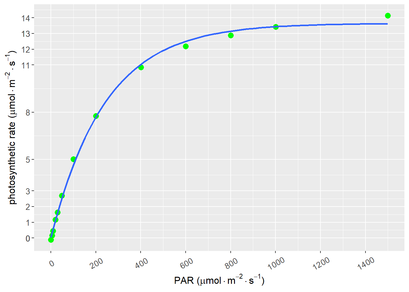
图 8.3: 指数模型拟合

表 8.3: 指数模型计算参数
	Estimate	Std. Error	t value	Pr(>\|t\|)
Am	13.6547568	0.1723363	79.233185	0.0000000
Ic	-0.5133438	2.3370250	-0.219657	0.8305573
b	0.0041183	0.0002012	20.467032	0.0000000

最终的数据拟结果如图 8.3 所示，拟合的参数及结果见表 8.3。

8.4 直角双曲线的修正模型

ZiPiao (2010) 直角双曲线修正模型的表达式如式 (8.5) 所示：

\[\begin{equation} P_{n} = \alpha \frac{1-\beta I}{1+\gamma I} I - R_{d} \tag{8.5} \end{equation}\]

其中，\(\beta\) 和 \(\gamma\) 为系数，\(\beta\)光抑制项，\(\gamma\)光饱和项，单位为 \(m^{2}\cdot s\cdot\mu mol^{-1}\)，其他参数与上文相同，因为该式 (8.5) 存在极值，因此，必然存在饱和光强和最大净光合速率，分别用式 (8.6) 和式 (8.7) 求得。

\[\begin{equation} I_{sat} = \frac{\sqrt{\frac{(\beta+\gamma)}{\beta}} - 1}{\gamma} \tag{8.6} \end{equation}\]

\[\begin{equation} P_{nmax} = \alpha\left(\frac{\sqrt{\beta+\gamma}-\sqrt{\beta}}{\gamma}\right)^{2}-R_{d} \tag{8.7} \end{equation}\]

该模型的优点为拟合结果中光饱和点和最大净光合速率均接近实测值，还可以拟合饱和光强之后光合速率随光强下降段的曲线。

8.4.1 直角双曲线修正模型的实现

library(minpack.lm)

# 读取数据，同fitaci数据格式
lrc <- read.csv("./data/lrc.csv")
lrc <- subset(lrc, Obs > 0)

# 光响应曲线没有太多参数，
# 直接调出相应的光强和光合速率
# 方便后面调用
lrc_Q <- lrc$PARi
lrc_A <- lrc$Photo 

# 模型的拟合
lrcnls <- nlsLM(lrc_A ~ alpha * ((1 - 
              beta*lrc_Q)/(1 + gamma * lrc_Q)) * lrc_Q - Rd,
                start=list(alpha = 0.07, beta = 0.00005,
                           gamma=0.004, Rd = 0.2)
                )
fitlrc_mrec <- summary(lrcnls)

# 饱和点计算
Isat <-  (sqrt((fitlrc_mrec$coef[2,1] + fitlrc_mrec$coef[3,1])/
              fitlrc_mrec$coef[2,1]) -1)/fitlrc_mrec$coef[3,1]
# 补偿点计算
Ic <- (
  -(fitlrc_mrec$coef[3, 1] * fitlrc_mrec$coef[4, 1] - 
  fitlrc_mrec$coef[1, 1]) - sqrt((fitlrc_mrec$coef[3, 1] * 
  fitlrc_mrec$coef[4, 1] - fitlrc_mrec$coef[1, 1])^2- 
  (4 * fitlrc_mrec$coef[1, 1] * fitlrc_mrec$coef[2, 1] * 
  fitlrc_mrec$coef[4, 1])))/
  (2*fitlrc_mrec$coef[1,1]*fitlrc_mrec$coef[2,1])

## 拟合图形
library(ggplot2)
light <- data.frame(lrc_Q = lrc$PARi, lrc_A = lrc$Photo)

p <- ggplot(light, aes(x = lrc_Q, y = lrc_A))

p1 <- p + 
  geom_point(shape = 16, size = 3, color = "green") + 
  geom_smooth(method="nls", formula = 
   y ~ alpha * ((1 - 
              beta*x)/(1 + gamma * x)) * x - Rd, 
    se = FALSE, method.args = list(
    start = c(alpha = 0.07, beta = 0.00005,
              gamma=0.004, Rd = 0.2), 
    aes(x =lrc_Q, y = lrc_A, 
    color='blue', size = 1.2))
  ) +
  labs(y=expression(paste("photosynthetic rate  ", 
          "(", mu, mol%.%m^-2%.%s^-1, ")")), 
       x=expression(paste("PAR ", 
           "(", mu, mol%.%m^-2%.%s^-1, ")")))


# 自定义坐标轴
p1 + scale_x_continuous(breaks = seq(0, 2100, by = 200)) +  
  scale_y_continuous(breaks= round(light$lrc_A)) +
   theme(axis.text.x  = element_text(
    size = 10, angle=30, vjust=0.5), 
    axis.text.y = element_text(size = 10),
    axis.title.x = element_text(size = 12, face = 'bold'),
    axis.title.y = element_text(size = 12, face = 'bold')
  )

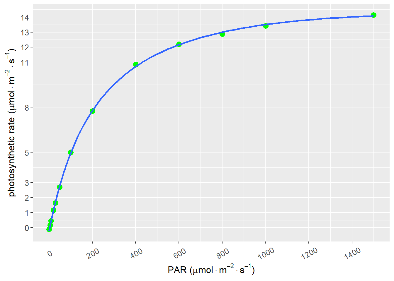
图 8.4: 直角双曲线修正模型拟合

表 8.4: 直角双曲线修正模型计算参数
	Estimate	Std. Error	t value	Pr(>\|t\|)
alpha	0.0730858	0.0021209	34.460183	0.0000000
beta	0.0000501	0.0000133	3.776115	0.0043751
gamma	0.0040622	0.0001955	20.773916	0.0000000
Rd	0.2156186	0.0543505	3.967190	0.0032685

尽管修正模型可以方便的计算饱和点和补偿点，但如同 Lobo et al. (2013) 所指出，双曲线模型对其结果的计算常有超出生态学意义范围的值¹³，因此对模型的选择不能一概而论，需根据实际情况而选择。

参考文献

Baly, EC. 1935. “The Kinetics of Photosynthesis.” Proceedings of the Royal Society of London Series B (Biological Sciences), no. 117: 218–39.

Huang, HY, XY Dou, PY Sun, B Deng, GJ Wu, and CL Peng. 2009. “Comparison of Photosynthetic Characteristics in Two Ecotypes of Jatropha Curcas in Summer.” Acta Ecologica Sinica, no. 29: 2861–67.

Lobo, F. De A., M. P. De Barros, H. J. Dalmagro, Â. C. Dalmolin, W. E. Pereira, É. C. de Souza, G. L. Vourlitis, and C. E. Rodríguez Ortíz. 2013. “Fitting Net Photosynthetic Light-Response Curves with Microsoft Excel a Critical Look at the Models.” Photosynthetica 51 (3): 445–56.

Prado, C. H., and J. A. P. V. De Moraes. 1997. “Photosynthetic Capacity and Specific Leaf Mass in Twenty Woody Species of Cerrado Vegetation Under Field Conditions.” Photosynthetica 33 (1): 103–12.

Thornley, J H M. 1976. “Mathematical Models in Plant Physiology.” London: Academic Press.

Zhang, XS, SH Shen, and J Song. 2009. “The Vertical Distribution of Cotton Leaf Nitrogen Content and Photosynthetic Characteristics in the North China Plain.” Acta Ecologica Sinica, no. 29: 1893–98.

ZiPiao, YE. 2010. “A Review on Modeling of Responses of Photosynthesis to Light and \(CO_2\).” Chinese Journal of Plant Ecology, no. 06.

第 8 章 光响应曲线的拟合